User login
Introduction: Biostatistics and epidemiology lecture series, part 1
Physicians are inundated with clinical research findings that potentially impact patient care. Evaluating the strength and clinical application of research results requires an understanding of the underlying biostatistics and epidemiological principles.
The articles in this supplement are based on a series of lectures originally developed for fellows in pulmonary and critical care medicine to provide them with the tools to transform a scientific or clinical question into research projects, and then pursue the answer to their question with the appropriate methods. The same skills also enable them to appraise the published literature in a systematic and rigorous manner.
Each topic in the series began with a presentation and discussion of statistical principles and methods, then moved to a practical module using the principles to appraise a specific publication. Participants in the course had an immediate opportunity to try the techniques, both to demonstrate understanding and to reinforce the concepts to each learner. The articles of this series follow the same outline, providing clinicians of all specialties the basic statistical tools to conduct and appraise clinical research, along with a sample article for practicing each statistical method presented.
This Cleveland Clinic Journal of Medicine supplement includes 3 lectures from the “Biostatistics and Epidemiology Lecture Series.” Dr. Stoller’s presentation, The Architecture of Clinical Research, describes the basic structure of clinical research and the nomenclature to understand trial design and sources of bias.
Building on those concepts, Dr. Chatburn’s lecture, Basics of Study Design: Practical Considerations, outlines the structured approach to develop a formal research protocol. How to identify a problem, expand the scope of it through a literature review, create a hypothesis, design a study, and an introduction to basic statistical methods are discussed.
And in Chi-square and Fisher’s Exact Tests, Dr. Nowacki introduces the statistical methodology of these 2 tests to assess associations between 2 independent categorical variables. The sample article illustrates step-by-step calculation of both the large sample approximation (chi-square) and exact (Fisher’s) methodologies providing insight into how these tests are conducted.
My hope is that these articles, and future installments based on forthcoming lectures, are helpful to physicians both in conducting their own research and in evaluating the research of others

The architecture of clinical research
I am flattered to present the inaugural talk in the biostatistics and clinical research design series on the architecture of clinical research. This content is based on the teachings of my mentor, Dr. Alvan Feinstein, who together with Dr. David Sackett, is credited with pioneering clinical epidemiology. Dr. Feinstein was a Sterling Professor at the Yale School of Medicine. His main opus of work is a book called, Clinical Epidemiology: The Architecture of Clinical Research.1 This paper is named in credit to Dr. Feinstein’s enormous contribution. I will review some important terms defined by Dr. Feinstein to provide the background necessary for the remainder of the talks in this series.
To start, I will frame this topic by asking the following question: Why do we do research? I’ll talk about the basic structure of research studies and provide a taxonomy, as Dr. Feinstein would say, a nomenclature with which to understand trial design and the sources of bias in those trials. Then, I will discuss these sources of bias in detail using the taxonomy that Dr. Feinstein described in his aforementioned book. Finally, I will share with you some examples of bias in clinical trials to help you better understand these concepts.
Now, the answer to the basic question posed above is: basically, we do cause-and-effect research to establish the causality of a risk factor or the efficacy of a therapy. Does cigarette smoking cause lung cancer? Does taking hydrochlorothiazide help systemic hypertension? Does air pollution worsen asthma? Does supplemental oxygen help patients with chronic obstructive pulmonary disease (COPD)?
Cause-and-effect research can be subsumed under 2 broad issues: causal risk factors and therapeutic efficacy. In his review of early false understandings in medicine that were based on anecdotal observation alone, Thomas cites many examples—“the undue longevity of useless and even harmful drugs can be laid at the door of authority,” ie, empiricism, lack of rigorous research.2 The field is full of these: yellow fever causality, the value of cupping, and even intermittent mandatory ventilation when it was described by John Downs in 1973 and touted as a superior mode for weaning patients from mechanical ventilation.3 Twenty-five years later, randomized controlled trials by Brochard et al4 indicated not only that intermittent mandatory ventilation was not the best mode to wean but was, in fact, the worst mode for weaning patients from mechanical ventilation compared with either pressure support or spontaneous breathing trials. Many more examples exist to demonstrate the false understandings that can be ascribed to lack of rigorous study or evidence in medicine.

Before systematically exploring the sources of bias in Feinstein’s construct, let us define some very basic terms from his book. Dr. Feinstein talks about the baseline state, which refers to the group of patients under study who are culled from a larger population to whom the results are intended to be applied (Figure 1).1 This baseline group is hopefully representative of this larger target population. As a nod to the later discussion, Dr. Feinstein would call bias introduced by unusual assembly of the study population from the larger intended population as “assembly bias.” So, if the group under study is not representative of either the patients you see or the world of patients with this condition or if there is something special or distinctively nonrepresentative about the study population, then the results may be subject to “assembly bias.” Assembly bias can compromise the so-called “external” validity of the study—its ability to be applied to populations beyond the study group.
Having assembled a baseline group for study, that group is classically allocated to 1 of 2 (or sometimes more than 2) compared therapies. In a controlled trial, patients can be allocated using a variety of strategies, including randomization. Using the paradigm diagram (Figure 1, which considers a 2-arm trial), patients are allocated to 1 of 2 compared groups—group A and group B. Then, in a treatment trial, 1 group receives the principal maneuver, which is the drug or intervention under study—for example, supplemental oxygen for patients with COPD. The comparative maneuver is allocated to group B, which also receives all the other treatments (called “co-maneuvers”) that are used to treat the condition under study. In a trial of supplemental oxygen for COPD evaluating lung function and exacerbation frequency as outcome measures, such co-maneuvers might include inhaled bronchodilators, inhaled corticosteroids, pulmonary rehabilitation, and Pneumovax vaccine. Ideally, these co-maneuvers are equally distributed between the compared groups (A and B).
So, in summary, we have a comparative maneuver, which is the nonadministration of supplemental oxygen in this proposed trial of supplemental oxygen in COPD, the principal maneuver—administration of oxygen—and all the co-maneuvers that are ideally equally distributed between both groups. This balanced distribution of co-maneuvers between the compared groups helps to ensure that any differences in the study outcome measures (ie, what is counted as the main impact of the intervention under study) can be solely attributed to the principal maneuver. When this condition—that the difference in outcomes can be reliably ascribed to the study intervention—is satisfied, the study is felt to be “internally” valid. As we will see, ensuring internal validity requires freedom from the many sources of what Dr. Feinstein calls “internal bias.”
Back to basic terms: “cohort” in Dr. Feinstein’s language is a group that shares common traits and is followed forward in a longitudinal study. The “outcome measure” is self-evident—it is what is being measured, with the “primary outcome” being the pre-defined measure that is considered the most important (and ideally most clinically relevant) impact of the study intervention. Later in this series of lectures, there will be discussions of power calculations and the so-called “effect size”—the magnitude of effect that the intervention is expected to produce and that is ideally deemed clinically important.
An important consideration in designing a trial is to define and declare the primary outcome measure carefully because defining the primary outcome measure has important implications for the study. I will provide an example from the alpha-1 antitrypsin deficiency literature. Some of you have probably read what has been called the RAPID trial.5 RAPID was a trial of augmentation therapy vs placebo in patients with severe alpha-1 antitrypsin deficiency. The primary outcome measure (which was pre-negotiated with the US Food and Drug Administration [FDA]) was computer tomography (CT) lung density determined at functional residual capacity (FRC) and total lung capacity (TLC). The trial failed to achieve statistical significance in regard to CT lung density, although the study authors argued that CT density measurements made at TLC were more reproducible than those made at FRC. When the results were analyzed by TLC alone, the results were statistically significant, but when they were analyzed with FRC and TLC combined, they were not. In the end, based on the pre-negotiated primary outcome measure of CT density based on both FRC and TLC, the FDA rejected the proposal for a label change to say that augmentation therapy slowed the loss of lung density even though the weight of evidence was clearly in its favor. This case exemplifies just how critical the choice of primary outcome measure can be.

The wash-out period refers to an interval in a subset of randomized trials called “crossover trials” in which the primary intervention is discontinued and the patient returns to his baseline state before the comparative maneuver is then implemented (Figure 2).6 In order to perform a crossover trial, it is important that the effects of the initial intervention can “wash out” or be fully extinguished. So, for example, in trials of radiation therapy vs surgery, it is impossible to do a crossover trial because the effects of radiation can never completely wash out nor can those of surgery, which are similarly permanent. For example, we cannot replace the colon once it is resected for cancer or replace the appendix once removed. Therefore, producing a wash-out requires some very specific pharmacokinetic and pharmacodynamic features in order for a crossover trial to be considered. Later talks in this series will discuss the enhanced statistical power of a crossover trial, where one is comparing every patient to him or herself rather than to another patient.
So, there is always an appetite to do a crossover trial as long as the criteria for wash-out can be met, namely again that the primary intervention can dissipate completely to the baseline state before the alternative intervention is implemented.
“Placebo” is a fairly self-evident and well-understood term; placebo refers to the administration of a maneuver in a way that is identical to the principal maneuver except that the placebo is not expected to exert any clinical effect.
“Blinding” is the unawareness of either the investigator or of the patient to which the intervention is being administered. “Single-blinding” refers to the condition in which either the study or the investigator (but not both) is unaware, and “double-blinding” refers to the condition in which both the subjects and the investigators are unaware. There can be some subtle issues that compromise whether the patient is aware of the intervention that he or she is receiving and that can potentially condition the patient’s response, particularly if there is any subjective component of the assessment of the outcome. So, blinding is important.
With these terms describing the elements of a clinical study now described, let us turn to the types of studies that comprise clinical research. The first group of study types is what Dr. Feinstein called descriptive studies—studies that simply describe phenomena without comparison to a control group. As an example of a descriptive study, Sehgal et al7 recently described the workup of a focal, segmental pneumonia in a patient taking pembrolizumab for lung cancer. In this paper, there were four other cases of focal pneumonia accompanying pembrolizumab use that were assembled from the literature, making this descriptive paper a so-called case series. A “case series” differs from a “single case report,” which reports a single patient experience. Though limited in their ability to establish cause and effect, case reports and case series can help researchers develop proof of principle, so I would not discount the value of case reports.8
I can cite a case report from of my own experience that demonstrates this point. In 1987, I saw a patient from Buffalo who had primary biliary cirrhosis and the hepatopulmonary syndrome (HPS). She was so debilitated by her HPS that she could not stand up without desaturating severely. Although she had normal liver synthetic function, she was severely debilitated by her HPS and the decision was made to offer her a liver transplant, which, at that time, was considered to be relatively contraindicated. Much to everyone’s amazement and satisfaction, her HPS completely resolved after the transplant surgery. Her oxygenation and alveolar-arterial oxygen gradient normalized, and her clubbing resolved. We reported this in a case report, which began to affect the way people thought about the feasibility of liver transplant for the HPS.8 The lesson is: do not underestimate the power of a thoughtful case report.
The second group of research study types is called “cohort studies,” in which one actually compares outcomes between 2 groups in the study. Cohort studies fall into the bucket of either “observational cohort studies,” in which allocation to the compared maneuvers is not performed by randomization but by any other strategy, and “randomized trials.” In observational studies, allocation could occur through physician choice, as when the physician prescribes a treatment to 1 group but not another, or by patient choice or circumstance. For example, an observational cohort study of the risk of cigarette smoking would compare outcomes between smokers and non-smokers where the patient choses to smoke under his/her own volition. Alternatively, the circumstances of an exposure could allocate someone to the principal maneuver, as when we are studying the effect of exposure to World Trade Center dust in the firefighters who responded or of exposure to nuclear radiation in Hiroshima survivors. These are examples of observational cohort studies that compare exposed individuals to unexposed individuals, where the exposure did not occur by randomization but by choice or unfortunate circumstance.
In contrast to observational studies, allocation in randomized trials occurs through a formal process. Randomization has the specific purpose of attempting to ensure that patients are allocated to 2 comparative groups from the baseline group with comparable risk for developing the outcome measure. When randomization is effective, differences in study outcomes can be reliably ascribed to the intervention rather than to differences in the baseline susceptibility of the compared groups.
While randomization is an excellent strategy to ensure baseline similarity between compared groups, randomization can fail, and its effectiveness must be checked. Specifically, in a randomized trial, it is customary to examine the compared groups at baseline on all features that can affect the likelihood of developing the outcome measure. If the groups turn out to be dissimilar at baseline in an important way, then the study is at risk for bias, which is specifically called “susceptibility bias” in Feinstein’s construct. Obviously, the larger number of baseline clinical and demographic features that can condition the likelihood of developing the outcome measure, the more difficult it is to achieve baseline similarity between compared groups and the more important it becomes to ensure that randomization has been effective. In this circumstance, larger numbers of participants in both compared groups are generally needed. More about susceptibility bias later.
There are generally 2 types of randomized trials: the so-called “parallel controlled trials” in which each group receives either the principal or the comparative maneuver and is followed and “crossover trials” in which each compared group receives both the principal maneuver and the co-maneuver at different times after an effective wash-out period. Wash-out was discussed above. Figure 2 shows an example of a crossover trial examining the effects of terbutaline on diaphragmatic function.6 The investigators administered terbutaline for a week, measured transdiaphragmatic pressures, gave the patient a terbutaline vacation (the “wash-out period”), and then crossed over those patients who were initially receiving terbutaline to placebo and initial placebo recipients to terbutaline, having remeasured diaphragmatic function after the wash-out period to assure that the patient’s diaphragmatic function prior to the second crossover was identical to his/her baseline state. If this return to baseline is accomplished, then the criteria from effective wash-out are satisfied.


As we begin to talk about sources of bias, consider a study in which we compare survival of patients allocated to surgery vs nonsurgical therapy for lung cancer (Figure 3).1 This study is subject to the first type of so-called “internal bias” in the Feinsteinian construct—so-called “selection bias.” For example, all patients treated surgically were considered healthy enough by their doctors to undergo surgery, whereas patients treated without surgery may have been deemed inoperable because of comorbidities, lung dysfunction, cardiac dysfunction, and so on. If the results of such a comparison show that the mortality rate among surgical patients in this study was lower, the question then becomes: is the improved survival in surgical candidates due to the superior efficacy of surgery vs other therapy or was the enhanced survival due to the surgical patients being healthier to begin with? You can intuitively sense that the answer to this question is that the enhanced survival may be due to the better health of patients treated surgically rather than to the surgery itself because of how the patients were selected to receive it. So, this is a simple example of what Dr. Feinstein would call “susceptibility bias.” Susceptibility bias occurs when the 2 baseline groups are not comparably at risk or susceptible to developing the outcome measure, leading the naïve investigator in this specific example to attribute the difference in outcomes to the superiority of surgery when in fact it may have nothing to do with the surgery vs. the other maneuver. When susceptibility bias is in play, the difference between the outcomes in the compared groups could be attributed to the baseline imbalance of the groups rather than to the principal maneuver itself.
Turning back to the taxonomy of bias, there are four types that can threaten internal validity—“susceptibility,” “performance,” “detection,” and “transfer” bias—and 1 type of bias (called “external bias”) that can affect the generalizability of the study called “assembly bias” (Table 1).

Figure 4 shows where these various sources of bias appear in the architecture of a clinical trial. As just discussed, susceptibility bias affects the baseline state and the comparability of the groups. Performance bias relates to how effective and how comparably the co-maneuvers are given and whether the primary intervention is potent enough to affect an outcome. Both transfer and detection bias operate in detecting the outcome, especially regarding the rigor and frequency with which they are investigated. Transfer bias has to do with selective loss to follow-up of those included in the trial. If there is a systematic reason for loss to follow-up that is related to the impact of the intervention, then the study is at risk for transfer bias. For example, in a randomized trial of drug A vs placebo for pneumonia, if drug A is effective but all the drug A recipients fail to follow-up because they feel too good to return for follow-up, then transfer bias could be causing the study to show nonefficacy even though the drug works. So, if those who respond favorably are systematically lost to follow-up, and if all the patients who felt lousy wanted to see the doctor and came back for follow-up, such transfer bias would bias towards nonefficacy. Specifically, only patients remaining in the trial would be those who failed to respond and that would dilute any difference between the 2 groups despite the active efficacy of drug A.
Hopefully, you are already beginning to get a sense that one has to be extremely disciplined in thinking about each of these sources of bias because they can have some very subtle nuances in randomized trials that can easily escape attention.
Returning to sources of bias, let’s consider the second type of bias, “performance bias.” Performance bias relates to the administration of the compared maneuvers—the primary or principal maneuver, compared with the comparative maneuver. Performance bias can occur when the main maneuver is not administered adequately or when the co-maneuvers are administered in an imbalanced way between the compared groups. Consider the example of the Long-Term Oxygen Treatment Trial (LOTT) trial, which compared use of supplemental oxygen with no supplemental oxygen in patients with stable COPD and resting or exercise-induced moderate desaturation.9 The principal outcome measure of LOTT was all-cause hospitalization or death. In such a study, many potential sources of performance bias exist. For example, performance bias might exist if none of the patients allocated to oxygen actually used supplemental oxygen. Alternately, to the extent that use of inhaled corticosteroids or antimuscarinic agents lessens the risk of COPD exacerbation, performance bias could occur if use of these co-maneuvers was imbalanced between the compared groups. As a specific extreme circumstance, if all patients in the nonoxygen group used these inhalers but none of the patients in the oxygen group did, then a lack of difference between exacerbation frequency could be related to this imbalance in co-maneuvers (a form of performance bias) rather than to the lack of efficacy of supplemental oxygen.
“Compliance bias” is a subset of performance bias which occurs when 2 conditions are satisfied: (1) the main maneuver is not administered adequately, and (2) the investigator is unaware of that nonreceipt so that this cannot be accounted for in interpreting the study results. For example, if a drug has efficacy but if no one in the treatment arm of the trial takes the drug, the absence of a difference in outcomes between the compared groups will be ascribed to nonefficacy, whereas “compliance bias” (ie, no one actually took the drug) could actually be the cause. Ideally, randomized studies should be evaluated on an “intention to treat” basis irrespective of compliance, but there is an analytic approach called “per protocol” analysis in which you can analyze the results according to whether the patient actually used the intervention in an effective way. “Per protocol” analysis is a secondary analysis of the primary results but it can nonetheless help determine whether the negative result is likely related to noncompliance or not.
A third type of internal bias, “detection bias,” is fairly straightforward. Detection bias is related to how avidly and how comparably the outcomes are measured between the 2 compared groups. Let’s say that you are conducting a trial of a new antibiotic and the primary outcome is colony counts on petri dishes of plated collected specimens. If the technicians who read the petri dish counts are unblinded, they may look at the colony counts with a biased eye, seeing fewer colonies on plates collected from patients receiving the antibiotic.
Overall, detection bias occurs when outcomes are ascertained or detected unequally between the compared groups, and detection bias can involve any of the following: is there comparable surveillance of the 2 groups for analysis of the outcome measure? Are the diagnostic tests comparably performed in both groups and is the interpretation comparably unbiased with equipoise? Investigators who know which patients are receiving an active drug and those who are not could experience subliminal bias that renders them more likely to find that the drug under study is efficacious.
Depending on the principal study maneuver, ensuring blinding can be challenging. To demonstrate this point, let’s consider the example of conducting a randomized control trial of Vicks VapoRub. Vicks VapoRub is an old product that smells like wintergreen and that mothers used to rub on the chests of their infants in the hope of speeding recovery from colds and bronchitis episodes. It was felt that the distinctive smell of the product was materially related to wintergreen, which gives rise to the odor. So, imagine a randomized trial of Vicks VaporRub. A trial is designed in which sick children receive Vicks VapoRub on their chest and others receive a placebo rub that lacks the distinctive wintergreen odor. But, the odor itself is felt to be related to how Vicks VapoRub actually works. Thus, it is the odor itself that creates the blinding challenge here.
The primary outcomes in this study are the duration of the child’s cold symptoms, as ascertained by pediatricians actually examining the children. So, pediatricians would come and listen to the infants’ chests: “Yeah, this chest is clear, but this other infant is still full of rhonchi,” and they would ascertain the outcome measure in this way. So, my blinding question to you is: how do you blind a trial of Vicks VapoRub given the conditions described? Namely, you put the VapoRub on the chest, it smells and the smell is the intervention—how do you blind such a trial?
The clever answer is that you should put Vicks VapoRub on the upper lips of all the examiners, so what they smell is Vicks VapoRub independent of whether the child they are examining also has the Vicks VapoRub or placebo on their chest. In this way, single blinding of the examiners is preserved and detection bias is averted. It is important to point out that double blinding could also be achieved by placing Vicks VapoRub on the child’s upper lip, but there is little reason to suspect that the infants being studied have a bias related to whether they smell the Vicks VapoRub.
The fourth potential source of internal bias is called “transfer bias.” Transfer bias is the selective loss to follow-up of patients from 1 of the 2 compared groups in the trial for a systematic reason. By systematic, I mean that that the drop-out is associated with the development of the outcome event or some impact of the intervention regarding the likelihood to develop the outcome event. As an example, if all patients respond favorably to a drug and everybody fails to follow up because they feel too good to come back, then that would bias the study towards nonefficacy even in the face of an efficacious intervention.
Finally, let’s consider a source of bias that can affect the “external validity,” or the generalizability of the study results to populations other than that included in the study itself. Dr. Feinstein calls this 5th type of bias “assembly bias” (Table 1).1 Assembly bias occurs when the results of the study cannot be reliably applied to populations outside the study itself.
For example, if I screen patients during a study of digoxin for heart rate control in atrial fibrillation, I could establish whether the subject was compliant or not by checking his/her serum digoxin levels. Serum levels of 0 indicate that the patient has not taken the digoxin. If I include a run-in period for the trial—an interval before the actual study when I am assessing potential subjects’ eligibility to participate—and check serum digoxin levels to include only patients who are shown to be taking the drug, then I am screening for study inclusion on compliance. In this way, I will have assembled a population that is highly compliant so that I can truly assess whether digoxin has efficacy in controlling the heart rate in patients with atrial fibrillation. At the same time, this study population is not highly representative of the population of patients with atrial fibrillation at large, because we know that rates of drug noncompliances may be as high as 30% to 40%. So, culling a population with run-in periods on demonstrated compliance criteria may be very important to assess efficacy (ie, whether the drug works), but this design will trade off on the effectiveness of the drug (ie, which asks the question “does the drug work in actual practice?”). This is because, in the yin-yang between assessing efficacy and assessing effectiveness, the focus on assessing efficacy naturally undermines the ability to assess whether the drug works in real-world conditions.
As another example of potential assembly bias, let’s say you are studying an antihypertensive drug at a Veterans Administration (VA) hospital, where most veterans are men. But you are treating women in your practice and wonder whether the drug, which works in a predominately male population, will work in your female patients. So, there could be assembly bias in applying the results of a VA study to a non-VA predominantly female population.
Having now described the design of clinical trials and the major sources of bias, let’s apply this thinking to the earliest clinical trial. James Lind, a British Naval officer, was credited with conducting the first clinical trial of citrus fruits for scurvy while sailing on the ship Salisbury in 1747.2 The question that Lind addressed was “does citrus fruit treat and prevent scurvy?” In describing this trial, Lind stated “I took 12 patients with scurvy, these patients were as similar as I could have them, had one diet common to all.” As you read this through your new Feinsteinian bias lens, Lind is addressing 2 potential sources of bias, namely, susceptibility bias and performance bias. In trying to make the “cases as similar as I could have them,” he is trying to avoid susceptibility bias and in “providing one diet common to all,” he is trying to avoid performance bias.
In terms of the intervention in this trial, these 12 patients were allocated in pairs to several interventions: a quart of cider a day, 25 drops of elixir of vitriol 3 times a day on an empty stomach, 2 spoonsful of vinegar 3 times a day on an empty stomach, ½ pint a day of sea water, 2 oranges and 1 lemon given every day, and a “bigness of nutmeg” 3 times per day. In describing the outcome of the trial, Lind states “the consequence was that the most sudden and visible good effects were perceived from the use of oranges and lemons; one of those who had taken them, being at the end of 6 days fit for duty. The spots were not indeed at that time quite off his body, nor his gums sound, but without any other medicine then a gargarism of elixir vitriol, he became quite healthy before we came into Plymouth which was on the 16th of June. The other was the best recovered of any in his condition; and being now deemed pretty well, was appointed nurse to the rest of the sick.”
In analyzing this trial, we could characterize it as a parallel controlled trial. Whether the allocation was done by randomization is not clear, but it was certainly an observational cohort study in that there were concurrent controls who were treated as similarly as possible except for the principal maneuver, which was the administration of citrus fruit. Already mentioned was the attention to averting susceptibility and performance bias. There was no evidence of compliance bias as the interventions were enforced, nor was there evidence of transfer bias because all subjects who were enrolled in the study completed the study because they were a captive group on a sailing ship. Finally, the likelihood of assembly bias seems small, as these sailors seemed to be representative of victims of scurvy in general, namely in being otherwise deprived of access to citrus fruits.
In terms of the statistical results of this study, subsequent analysis of the research showed that the impact of lemons and oranges was dramatic and showed a trend (P = .09) towards statistical significance. Notwithstanding the lack of a P < .05, Dr. Feinstein would likely say that this study satisfied the “intra-ocular test” in that the efficacy of the citrus fruit was so dramatic that it “hit you between the eyes.” He often argued that the widespread practice of prescribing penicillin for pneumococcal pneumonia was not based on the results of a convincing randomized controlled trial because the efficacy of penicillin in that setting was so dramatic that a randomized trial was not necessary (and potentially even unethical if the condition of “intra-ocular” efficacy was satisfied).
The final question to address in this lecture is whether randomized controlled trials, for all their rigor, always produce more reliable results than observational studies. This issue has been addressed by several authors.10–12 Sacks et al10 contended in 1983 that observational studies systematically overestimate the magnitude of association between exposure and outcome and therefore argued that randomized trials were more reliable than observational studies. Subsequent analyses tended to challenge this view.11,12 Specifically, Benson and Hartz11 compared the results of 136 reports regarding 19 different therapies that were studied between 1985 and 1998. In only 2 of the 19 analyses did the treatment effects in the observational studies fall outside the 95% confidence interval for the randomized controlled trial results. In this way, these authors argued that observational studies generally are concordant with the results of randomized trials. They stated that “our finding that observational studies and randomized controlled trials usually produce similar results differs from the conclusions of previous authors. The fundamental criticism of observational studies is that unrecognized confounding factors may distort the results. According to the conventional wisdom, this distortion is sufficiently common and unpredictable that observational studies are not liable and should not be funded. Our results suggested observational studies usually do provide valid information.”11
An additional analysis of this issue was performed by Concato et al,12 who identified 99 articles regarding 5 clinical topics. Again, the results from randomized trials were compared with those of observational cohort or case-controlled studies regarding the same intervention. The authors reported that “contrary to prevailing belief, the average results from well-designed observational studies did not systematically overestimate the magnitude of the associations between exposure and outcome as compared with the results of randomized, controlled trials on the same topic. Rather, the summary results of randomized, controlled trials and observational studies were remarkably similar.”12
On the basis of these studies, it appears that randomized control trials continue to serve as the gold standard in clinical research, but we must also recognize that circumstances often preclude the conduct of a randomized trial. As an example, consider a randomized trial of whether cigarette smoking is harmful, which, given the strong suspicion of harm, would be unethical in that patients cannot be randomized to smoke. Similarly, from the example before, a randomized trial of penicillin for pneumococcal pneumonia would be unethical because denying patients in the placebo group access to penicillin would exclude them from access to a drug that has “intra-ocular” efficacy. In circumstances like these, well-performed observational studies that are attentive to sources of bias can likely produce comparably reliable results to randomized trials.
In the end, of course, the interpretation of the study results requires the reader’s careful attention to potential sources of bias that can compromise study validity. The hope is that with Dr. Feinstein’s framework, you can be better equipped to think critically about study results that you review and to keenly ascertain whether there is any threat to internal or to external validity. Similarly, as you go on to design clinical trials yourselves, you can pay attention to these potential sources of bias that, if present, can compromise the reliability of the study conclusions internally or their applicability to patients outside of the study.
- Feinstein AR. Clinical Epidemiology: The Architecture of Clinical Research. Philadelphia, PA: WB Saunders; 1985.
- Thomas DP. Experiment versus authority: James Lind and Benjamin Rush. N Engl J Med 1969; 281:932–934.
- Downs JB, Klein EF Jr, Desautels D, Modell JH, Kirby RR. Intermittent mandatory ventilation: a new approach to weaning patients from mechanical ventilators. Chest 1973; 64:331–335.
- Brochard L, Rauss A, Benito S, et al. Comparison of three methods of gradual withdrawal from ventilatory support during weaning from mechanical ventilation. Am J Respir Crit Care Med 1994; 150:896–903.
- Chapman KR, Burdon JGW, Piitulainen E, et al; on behalf of the RAPID Trial Study Group. Intravenous augmentation treatment and lung density in severe 1 antitrypsin deficiency (RAPID): a randomised, double-blind, placebo-controlled trial. Lancet 2015; 386:360–368.
- Stoller JK, Wiedemann HP, Loke J, Snyder P, Virgulto J, Matthay RA. Terbutaline and diaphragm function in chronic obstructive pulmonary disease: a double-blind randomized clinical trial. Br J Dis Chest 1988; 82:242–250.
- Sehgal S, Velcheti V, Mukhopadhyay S, Stoller JK. Focal lung infiltrate complicating PD-1 inhibitor use: a new pattern of drug-associated lung toxicity? Respir Med Case Rep 2016; 19:118–120.
- Stoller JK, Moodie D, Schiavone WA, et al. Reduction of intrapulmonary shunt and resolution of digital clubbing associated with primary biliary cirrhosis after liver transplantation. Hepatology 1990; 11:54–58.
- Albert RK, Au DH, Blackford AL, et al; for the Long-Term Oxygen Treatment Trial Group. A randomized trial of long-term oxygen for COPD with moderate desaturation. N Engl J Med 2016; 375:1617–1627.
- Sacks HS, Chalmers TC, Smith H Jr. Sensitivity and specificity of clinical trials: randomized v historical controls. Arch Intern Med 1983; 143:753–755.
- Benson K, Hartz AJ. A comparison of observational studies and randomized, controlled trials. N Engl J Med 2000; 342:1878–1886.
- Concato J, Shah N, Horwitz RI. Randomized, controlled trials, observational studies, and the hierarchy of research designs. N Engl J Med 2000; 342:1887–1892.
I am flattered to present the inaugural talk in the biostatistics and clinical research design series on the architecture of clinical research. This content is based on the teachings of my mentor, Dr. Alvan Feinstein, who together with Dr. David Sackett, is credited with pioneering clinical epidemiology. Dr. Feinstein was a Sterling Professor at the Yale School of Medicine. His main opus of work is a book called, Clinical Epidemiology: The Architecture of Clinical Research.1 This paper is named in credit to Dr. Feinstein’s enormous contribution. I will review some important terms defined by Dr. Feinstein to provide the background necessary for the remainder of the talks in this series.
To start, I will frame this topic by asking the following question: Why do we do research? I’ll talk about the basic structure of research studies and provide a taxonomy, as Dr. Feinstein would say, a nomenclature with which to understand trial design and the sources of bias in those trials. Then, I will discuss these sources of bias in detail using the taxonomy that Dr. Feinstein described in his aforementioned book. Finally, I will share with you some examples of bias in clinical trials to help you better understand these concepts.
Now, the answer to the basic question posed above is: basically, we do cause-and-effect research to establish the causality of a risk factor or the efficacy of a therapy. Does cigarette smoking cause lung cancer? Does taking hydrochlorothiazide help systemic hypertension? Does air pollution worsen asthma? Does supplemental oxygen help patients with chronic obstructive pulmonary disease (COPD)?
Cause-and-effect research can be subsumed under 2 broad issues: causal risk factors and therapeutic efficacy. In his review of early false understandings in medicine that were based on anecdotal observation alone, Thomas cites many examples—“the undue longevity of useless and even harmful drugs can be laid at the door of authority,” ie, empiricism, lack of rigorous research.2 The field is full of these: yellow fever causality, the value of cupping, and even intermittent mandatory ventilation when it was described by John Downs in 1973 and touted as a superior mode for weaning patients from mechanical ventilation.3 Twenty-five years later, randomized controlled trials by Brochard et al4 indicated not only that intermittent mandatory ventilation was not the best mode to wean but was, in fact, the worst mode for weaning patients from mechanical ventilation compared with either pressure support or spontaneous breathing trials. Many more examples exist to demonstrate the false understandings that can be ascribed to lack of rigorous study or evidence in medicine.
Before systematically exploring the sources of bias in Feinstein’s construct, let us define some very basic terms from his book. Dr. Feinstein talks about the baseline state, which refers to the group of patients under study who are culled from a larger population to whom the results are intended to be applied (Figure 1).1 This baseline group is hopefully representative of this larger target population. As a nod to the later discussion, Dr. Feinstein would call bias introduced by unusual assembly of the study population from the larger intended population as “assembly bias.” So, if the group under study is not representative of either the patients you see or the world of patients with this condition or if there is something special or distinctively nonrepresentative about the study population, then the results may be subject to “assembly bias.” Assembly bias can compromise the so-called “external” validity of the study—its ability to be applied to populations beyond the study group.
Having assembled a baseline group for study, that group is classically allocated to 1 of 2 (or sometimes more than 2) compared therapies. In a controlled trial, patients can be allocated using a variety of strategies, including randomization. Using the paradigm diagram (Figure 1, which considers a 2-arm trial), patients are allocated to 1 of 2 compared groups—group A and group B. Then, in a treatment trial, 1 group receives the principal maneuver, which is the drug or intervention under study—for example, supplemental oxygen for patients with COPD. The comparative maneuver is allocated to group B, which also receives all the other treatments (called “co-maneuvers”) that are used to treat the condition under study. In a trial of supplemental oxygen for COPD evaluating lung function and exacerbation frequency as outcome measures, such co-maneuvers might include inhaled bronchodilators, inhaled corticosteroids, pulmonary rehabilitation, and Pneumovax vaccine. Ideally, these co-maneuvers are equally distributed between the compared groups (A and B).
So, in summary, we have a comparative maneuver, which is the nonadministration of supplemental oxygen in this proposed trial of supplemental oxygen in COPD, the principal maneuver—administration of oxygen—and all the co-maneuvers that are ideally equally distributed between both groups. This balanced distribution of co-maneuvers between the compared groups helps to ensure that any differences in the study outcome measures (ie, what is counted as the main impact of the intervention under study) can be solely attributed to the principal maneuver. When this condition—that the difference in outcomes can be reliably ascribed to the study intervention—is satisfied, the study is felt to be “internally” valid. As we will see, ensuring internal validity requires freedom from the many sources of what Dr. Feinstein calls “internal bias.”
Back to basic terms: “cohort” in Dr. Feinstein’s language is a group that shares common traits and is followed forward in a longitudinal study. The “outcome measure” is self-evident—it is what is being measured, with the “primary outcome” being the pre-defined measure that is considered the most important (and ideally most clinically relevant) impact of the study intervention. Later in this series of lectures, there will be discussions of power calculations and the so-called “effect size”—the magnitude of effect that the intervention is expected to produce and that is ideally deemed clinically important.
An important consideration in designing a trial is to define and declare the primary outcome measure carefully because defining the primary outcome measure has important implications for the study. I will provide an example from the alpha-1 antitrypsin deficiency literature. Some of you have probably read what has been called the RAPID trial.5 RAPID was a trial of augmentation therapy vs placebo in patients with severe alpha-1 antitrypsin deficiency. The primary outcome measure (which was pre-negotiated with the US Food and Drug Administration [FDA]) was computer tomography (CT) lung density determined at functional residual capacity (FRC) and total lung capacity (TLC). The trial failed to achieve statistical significance in regard to CT lung density, although the study authors argued that CT density measurements made at TLC were more reproducible than those made at FRC. When the results were analyzed by TLC alone, the results were statistically significant, but when they were analyzed with FRC and TLC combined, they were not. In the end, based on the pre-negotiated primary outcome measure of CT density based on both FRC and TLC, the FDA rejected the proposal for a label change to say that augmentation therapy slowed the loss of lung density even though the weight of evidence was clearly in its favor. This case exemplifies just how critical the choice of primary outcome measure can be.
The wash-out period refers to an interval in a subset of randomized trials called “crossover trials” in which the primary intervention is discontinued and the patient returns to his baseline state before the comparative maneuver is then implemented (Figure 2).6 In order to perform a crossover trial, it is important that the effects of the initial intervention can “wash out” or be fully extinguished. So, for example, in trials of radiation therapy vs surgery, it is impossible to do a crossover trial because the effects of radiation can never completely wash out nor can those of surgery, which are similarly permanent. For example, we cannot replace the colon once it is resected for cancer or replace the appendix once removed. Therefore, producing a wash-out requires some very specific pharmacokinetic and pharmacodynamic features in order for a crossover trial to be considered. Later talks in this series will discuss the enhanced statistical power of a crossover trial, where one is comparing every patient to him or herself rather than to another patient.
So, there is always an appetite to do a crossover trial as long as the criteria for wash-out can be met, namely again that the primary intervention can dissipate completely to the baseline state before the alternative intervention is implemented.
“Placebo” is a fairly self-evident and well-understood term; placebo refers to the administration of a maneuver in a way that is identical to the principal maneuver except that the placebo is not expected to exert any clinical effect.
“Blinding” is the unawareness of either the investigator or of the patient to which the intervention is being administered. “Single-blinding” refers to the condition in which either the study or the investigator (but not both) is unaware, and “double-blinding” refers to the condition in which both the subjects and the investigators are unaware. There can be some subtle issues that compromise whether the patient is aware of the intervention that he or she is receiving and that can potentially condition the patient’s response, particularly if there is any subjective component of the assessment of the outcome. So, blinding is important.
With these terms describing the elements of a clinical study now described, let us turn to the types of studies that comprise clinical research. The first group of study types is what Dr. Feinstein called descriptive studies—studies that simply describe phenomena without comparison to a control group. As an example of a descriptive study, Sehgal et al7 recently described the workup of a focal, segmental pneumonia in a patient taking pembrolizumab for lung cancer. In this paper, there were four other cases of focal pneumonia accompanying pembrolizumab use that were assembled from the literature, making this descriptive paper a so-called case series. A “case series” differs from a “single case report,” which reports a single patient experience. Though limited in their ability to establish cause and effect, case reports and case series can help researchers develop proof of principle, so I would not discount the value of case reports.8
I can cite a case report from of my own experience that demonstrates this point. In 1987, I saw a patient from Buffalo who had primary biliary cirrhosis and the hepatopulmonary syndrome (HPS). She was so debilitated by her HPS that she could not stand up without desaturating severely. Although she had normal liver synthetic function, she was severely debilitated by her HPS and the decision was made to offer her a liver transplant, which, at that time, was considered to be relatively contraindicated. Much to everyone’s amazement and satisfaction, her HPS completely resolved after the transplant surgery. Her oxygenation and alveolar-arterial oxygen gradient normalized, and her clubbing resolved. We reported this in a case report, which began to affect the way people thought about the feasibility of liver transplant for the HPS.8 The lesson is: do not underestimate the power of a thoughtful case report.
The second group of research study types is called “cohort studies,” in which one actually compares outcomes between 2 groups in the study. Cohort studies fall into the bucket of either “observational cohort studies,” in which allocation to the compared maneuvers is not performed by randomization but by any other strategy, and “randomized trials.” In observational studies, allocation could occur through physician choice, as when the physician prescribes a treatment to 1 group but not another, or by patient choice or circumstance. For example, an observational cohort study of the risk of cigarette smoking would compare outcomes between smokers and non-smokers where the patient choses to smoke under his/her own volition. Alternatively, the circumstances of an exposure could allocate someone to the principal maneuver, as when we are studying the effect of exposure to World Trade Center dust in the firefighters who responded or of exposure to nuclear radiation in Hiroshima survivors. These are examples of observational cohort studies that compare exposed individuals to unexposed individuals, where the exposure did not occur by randomization but by choice or unfortunate circumstance.
In contrast to observational studies, allocation in randomized trials occurs through a formal process. Randomization has the specific purpose of attempting to ensure that patients are allocated to 2 comparative groups from the baseline group with comparable risk for developing the outcome measure. When randomization is effective, differences in study outcomes can be reliably ascribed to the intervention rather than to differences in the baseline susceptibility of the compared groups.
While randomization is an excellent strategy to ensure baseline similarity between compared groups, randomization can fail, and its effectiveness must be checked. Specifically, in a randomized trial, it is customary to examine the compared groups at baseline on all features that can affect the likelihood of developing the outcome measure. If the groups turn out to be dissimilar at baseline in an important way, then the study is at risk for bias, which is specifically called “susceptibility bias” in Feinstein’s construct. Obviously, the larger number of baseline clinical and demographic features that can condition the likelihood of developing the outcome measure, the more difficult it is to achieve baseline similarity between compared groups and the more important it becomes to ensure that randomization has been effective. In this circumstance, larger numbers of participants in both compared groups are generally needed. More about susceptibility bias later.
There are generally 2 types of randomized trials: the so-called “parallel controlled trials” in which each group receives either the principal or the comparative maneuver and is followed and “crossover trials” in which each compared group receives both the principal maneuver and the co-maneuver at different times after an effective wash-out period. Wash-out was discussed above. Figure 2 shows an example of a crossover trial examining the effects of terbutaline on diaphragmatic function.6 The investigators administered terbutaline for a week, measured transdiaphragmatic pressures, gave the patient a terbutaline vacation (the “wash-out period”), and then crossed over those patients who were initially receiving terbutaline to placebo and initial placebo recipients to terbutaline, having remeasured diaphragmatic function after the wash-out period to assure that the patient’s diaphragmatic function prior to the second crossover was identical to his/her baseline state. If this return to baseline is accomplished, then the criteria from effective wash-out are satisfied.
As we begin to talk about sources of bias, consider a study in which we compare survival of patients allocated to surgery vs nonsurgical therapy for lung cancer (Figure 3).1 This study is subject to the first type of so-called “internal bias” in the Feinsteinian construct—so-called “selection bias.” For example, all patients treated surgically were considered healthy enough by their doctors to undergo surgery, whereas patients treated without surgery may have been deemed inoperable because of comorbidities, lung dysfunction, cardiac dysfunction, and so on. If the results of such a comparison show that the mortality rate among surgical patients in this study was lower, the question then becomes: is the improved survival in surgical candidates due to the superior efficacy of surgery vs other therapy or was the enhanced survival due to the surgical patients being healthier to begin with? You can intuitively sense that the answer to this question is that the enhanced survival may be due to the better health of patients treated surgically rather than to the surgery itself because of how the patients were selected to receive it. So, this is a simple example of what Dr. Feinstein would call “susceptibility bias.” Susceptibility bias occurs when the 2 baseline groups are not comparably at risk or susceptible to developing the outcome measure, leading the naïve investigator in this specific example to attribute the difference in outcomes to the superiority of surgery when in fact it may have nothing to do with the surgery vs. the other maneuver. When susceptibility bias is in play, the difference between the outcomes in the compared groups could be attributed to the baseline imbalance of the groups rather than to the principal maneuver itself.
Turning back to the taxonomy of bias, there are four types that can threaten internal validity—“susceptibility,” “performance,” “detection,” and “transfer” bias—and 1 type of bias (called “external bias”) that can affect the generalizability of the study called “assembly bias” (Table 1).
Figure 4 shows where these various sources of bias appear in the architecture of a clinical trial. As just discussed, susceptibility bias affects the baseline state and the comparability of the groups. Performance bias relates to how effective and how comparably the co-maneuvers are given and whether the primary intervention is potent enough to affect an outcome. Both transfer and detection bias operate in detecting the outcome, especially regarding the rigor and frequency with which they are investigated. Transfer bias has to do with selective loss to follow-up of those included in the trial. If there is a systematic reason for loss to follow-up that is related to the impact of the intervention, then the study is at risk for transfer bias. For example, in a randomized trial of drug A vs placebo for pneumonia, if drug A is effective but all the drug A recipients fail to follow-up because they feel too good to return for follow-up, then transfer bias could be causing the study to show nonefficacy even though the drug works. So, if those who respond favorably are systematically lost to follow-up, and if all the patients who felt lousy wanted to see the doctor and came back for follow-up, such transfer bias would bias towards nonefficacy. Specifically, only patients remaining in the trial would be those who failed to respond and that would dilute any difference between the 2 groups despite the active efficacy of drug A.
Hopefully, you are already beginning to get a sense that one has to be extremely disciplined in thinking about each of these sources of bias because they can have some very subtle nuances in randomized trials that can easily escape attention.
Returning to sources of bias, let’s consider the second type of bias, “performance bias.” Performance bias relates to the administration of the compared maneuvers—the primary or principal maneuver, compared with the comparative maneuver. Performance bias can occur when the main maneuver is not administered adequately or when the co-maneuvers are administered in an imbalanced way between the compared groups. Consider the example of the Long-Term Oxygen Treatment Trial (LOTT) trial, which compared use of supplemental oxygen with no supplemental oxygen in patients with stable COPD and resting or exercise-induced moderate desaturation.9 The principal outcome measure of LOTT was all-cause hospitalization or death. In such a study, many potential sources of performance bias exist. For example, performance bias might exist if none of the patients allocated to oxygen actually used supplemental oxygen. Alternately, to the extent that use of inhaled corticosteroids or antimuscarinic agents lessens the risk of COPD exacerbation, performance bias could occur if use of these co-maneuvers was imbalanced between the compared groups. As a specific extreme circumstance, if all patients in the nonoxygen group used these inhalers but none of the patients in the oxygen group did, then a lack of difference between exacerbation frequency could be related to this imbalance in co-maneuvers (a form of performance bias) rather than to the lack of efficacy of supplemental oxygen.
“Compliance bias” is a subset of performance bias which occurs when 2 conditions are satisfied: (1) the main maneuver is not administered adequately, and (2) the investigator is unaware of that nonreceipt so that this cannot be accounted for in interpreting the study results. For example, if a drug has efficacy but if no one in the treatment arm of the trial takes the drug, the absence of a difference in outcomes between the compared groups will be ascribed to nonefficacy, whereas “compliance bias” (ie, no one actually took the drug) could actually be the cause. Ideally, randomized studies should be evaluated on an “intention to treat” basis irrespective of compliance, but there is an analytic approach called “per protocol” analysis in which you can analyze the results according to whether the patient actually used the intervention in an effective way. “Per protocol” analysis is a secondary analysis of the primary results but it can nonetheless help determine whether the negative result is likely related to noncompliance or not.
A third type of internal bias, “detection bias,” is fairly straightforward. Detection bias is related to how avidly and how comparably the outcomes are measured between the 2 compared groups. Let’s say that you are conducting a trial of a new antibiotic and the primary outcome is colony counts on petri dishes of plated collected specimens. If the technicians who read the petri dish counts are unblinded, they may look at the colony counts with a biased eye, seeing fewer colonies on plates collected from patients receiving the antibiotic.
Overall, detection bias occurs when outcomes are ascertained or detected unequally between the compared groups, and detection bias can involve any of the following: is there comparable surveillance of the 2 groups for analysis of the outcome measure? Are the diagnostic tests comparably performed in both groups and is the interpretation comparably unbiased with equipoise? Investigators who know which patients are receiving an active drug and those who are not could experience subliminal bias that renders them more likely to find that the drug under study is efficacious.
Depending on the principal study maneuver, ensuring blinding can be challenging. To demonstrate this point, let’s consider the example of conducting a randomized control trial of Vicks VapoRub. Vicks VapoRub is an old product that smells like wintergreen and that mothers used to rub on the chests of their infants in the hope of speeding recovery from colds and bronchitis episodes. It was felt that the distinctive smell of the product was materially related to wintergreen, which gives rise to the odor. So, imagine a randomized trial of Vicks VaporRub. A trial is designed in which sick children receive Vicks VapoRub on their chest and others receive a placebo rub that lacks the distinctive wintergreen odor. But, the odor itself is felt to be related to how Vicks VapoRub actually works. Thus, it is the odor itself that creates the blinding challenge here.
The primary outcomes in this study are the duration of the child’s cold symptoms, as ascertained by pediatricians actually examining the children. So, pediatricians would come and listen to the infants’ chests: “Yeah, this chest is clear, but this other infant is still full of rhonchi,” and they would ascertain the outcome measure in this way. So, my blinding question to you is: how do you blind a trial of Vicks VapoRub given the conditions described? Namely, you put the VapoRub on the chest, it smells and the smell is the intervention—how do you blind such a trial?
The clever answer is that you should put Vicks VapoRub on the upper lips of all the examiners, so what they smell is Vicks VapoRub independent of whether the child they are examining also has the Vicks VapoRub or placebo on their chest. In this way, single blinding of the examiners is preserved and detection bias is averted. It is important to point out that double blinding could also be achieved by placing Vicks VapoRub on the child’s upper lip, but there is little reason to suspect that the infants being studied have a bias related to whether they smell the Vicks VapoRub.
The fourth potential source of internal bias is called “transfer bias.” Transfer bias is the selective loss to follow-up of patients from 1 of the 2 compared groups in the trial for a systematic reason. By systematic, I mean that that the drop-out is associated with the development of the outcome event or some impact of the intervention regarding the likelihood to develop the outcome event. As an example, if all patients respond favorably to a drug and everybody fails to follow up because they feel too good to come back, then that would bias the study towards nonefficacy even in the face of an efficacious intervention.
Finally, let’s consider a source of bias that can affect the “external validity,” or the generalizability of the study results to populations other than that included in the study itself. Dr. Feinstein calls this 5th type of bias “assembly bias” (Table 1).1 Assembly bias occurs when the results of the study cannot be reliably applied to populations outside the study itself.
For example, if I screen patients during a study of digoxin for heart rate control in atrial fibrillation, I could establish whether the subject was compliant or not by checking his/her serum digoxin levels. Serum levels of 0 indicate that the patient has not taken the digoxin. If I include a run-in period for the trial—an interval before the actual study when I am assessing potential subjects’ eligibility to participate—and check serum digoxin levels to include only patients who are shown to be taking the drug, then I am screening for study inclusion on compliance. In this way, I will have assembled a population that is highly compliant so that I can truly assess whether digoxin has efficacy in controlling the heart rate in patients with atrial fibrillation. At the same time, this study population is not highly representative of the population of patients with atrial fibrillation at large, because we know that rates of drug noncompliances may be as high as 30% to 40%. So, culling a population with run-in periods on demonstrated compliance criteria may be very important to assess efficacy (ie, whether the drug works), but this design will trade off on the effectiveness of the drug (ie, which asks the question “does the drug work in actual practice?”). This is because, in the yin-yang between assessing efficacy and assessing effectiveness, the focus on assessing efficacy naturally undermines the ability to assess whether the drug works in real-world conditions.
As another example of potential assembly bias, let’s say you are studying an antihypertensive drug at a Veterans Administration (VA) hospital, where most veterans are men. But you are treating women in your practice and wonder whether the drug, which works in a predominately male population, will work in your female patients. So, there could be assembly bias in applying the results of a VA study to a non-VA predominantly female population.
Having now described the design of clinical trials and the major sources of bias, let’s apply this thinking to the earliest clinical trial. James Lind, a British Naval officer, was credited with conducting the first clinical trial of citrus fruits for scurvy while sailing on the ship Salisbury in 1747.2 The question that Lind addressed was “does citrus fruit treat and prevent scurvy?” In describing this trial, Lind stated “I took 12 patients with scurvy, these patients were as similar as I could have them, had one diet common to all.” As you read this through your new Feinsteinian bias lens, Lind is addressing 2 potential sources of bias, namely, susceptibility bias and performance bias. In trying to make the “cases as similar as I could have them,” he is trying to avoid susceptibility bias and in “providing one diet common to all,” he is trying to avoid performance bias.
In terms of the intervention in this trial, these 12 patients were allocated in pairs to several interventions: a quart of cider a day, 25 drops of elixir of vitriol 3 times a day on an empty stomach, 2 spoonsful of vinegar 3 times a day on an empty stomach, ½ pint a day of sea water, 2 oranges and 1 lemon given every day, and a “bigness of nutmeg” 3 times per day. In describing the outcome of the trial, Lind states “the consequence was that the most sudden and visible good effects were perceived from the use of oranges and lemons; one of those who had taken them, being at the end of 6 days fit for duty. The spots were not indeed at that time quite off his body, nor his gums sound, but without any other medicine then a gargarism of elixir vitriol, he became quite healthy before we came into Plymouth which was on the 16th of June. The other was the best recovered of any in his condition; and being now deemed pretty well, was appointed nurse to the rest of the sick.”
In analyzing this trial, we could characterize it as a parallel controlled trial. Whether the allocation was done by randomization is not clear, but it was certainly an observational cohort study in that there were concurrent controls who were treated as similarly as possible except for the principal maneuver, which was the administration of citrus fruit. Already mentioned was the attention to averting susceptibility and performance bias. There was no evidence of compliance bias as the interventions were enforced, nor was there evidence of transfer bias because all subjects who were enrolled in the study completed the study because they were a captive group on a sailing ship. Finally, the likelihood of assembly bias seems small, as these sailors seemed to be representative of victims of scurvy in general, namely in being otherwise deprived of access to citrus fruits.
In terms of the statistical results of this study, subsequent analysis of the research showed that the impact of lemons and oranges was dramatic and showed a trend (P = .09) towards statistical significance. Notwithstanding the lack of a P < .05, Dr. Feinstein would likely say that this study satisfied the “intra-ocular test” in that the efficacy of the citrus fruit was so dramatic that it “hit you between the eyes.” He often argued that the widespread practice of prescribing penicillin for pneumococcal pneumonia was not based on the results of a convincing randomized controlled trial because the efficacy of penicillin in that setting was so dramatic that a randomized trial was not necessary (and potentially even unethical if the condition of “intra-ocular” efficacy was satisfied).
The final question to address in this lecture is whether randomized controlled trials, for all their rigor, always produce more reliable results than observational studies. This issue has been addressed by several authors.10–12 Sacks et al10 contended in 1983 that observational studies systematically overestimate the magnitude of association between exposure and outcome and therefore argued that randomized trials were more reliable than observational studies. Subsequent analyses tended to challenge this view.11,12 Specifically, Benson and Hartz11 compared the results of 136 reports regarding 19 different therapies that were studied between 1985 and 1998. In only 2 of the 19 analyses did the treatment effects in the observational studies fall outside the 95% confidence interval for the randomized controlled trial results. In this way, these authors argued that observational studies generally are concordant with the results of randomized trials. They stated that “our finding that observational studies and randomized controlled trials usually produce similar results differs from the conclusions of previous authors. The fundamental criticism of observational studies is that unrecognized confounding factors may distort the results. According to the conventional wisdom, this distortion is sufficiently common and unpredictable that observational studies are not liable and should not be funded. Our results suggested observational studies usually do provide valid information.”11
An additional analysis of this issue was performed by Concato et al,12 who identified 99 articles regarding 5 clinical topics. Again, the results from randomized trials were compared with those of observational cohort or case-controlled studies regarding the same intervention. The authors reported that “contrary to prevailing belief, the average results from well-designed observational studies did not systematically overestimate the magnitude of the associations between exposure and outcome as compared with the results of randomized, controlled trials on the same topic. Rather, the summary results of randomized, controlled trials and observational studies were remarkably similar.”12
On the basis of these studies, it appears that randomized control trials continue to serve as the gold standard in clinical research, but we must also recognize that circumstances often preclude the conduct of a randomized trial. As an example, consider a randomized trial of whether cigarette smoking is harmful, which, given the strong suspicion of harm, would be unethical in that patients cannot be randomized to smoke. Similarly, from the example before, a randomized trial of penicillin for pneumococcal pneumonia would be unethical because denying patients in the placebo group access to penicillin would exclude them from access to a drug that has “intra-ocular” efficacy. In circumstances like these, well-performed observational studies that are attentive to sources of bias can likely produce comparably reliable results to randomized trials.
In the end, of course, the interpretation of the study results requires the reader’s careful attention to potential sources of bias that can compromise study validity. The hope is that with Dr. Feinstein’s framework, you can be better equipped to think critically about study results that you review and to keenly ascertain whether there is any threat to internal or to external validity. Similarly, as you go on to design clinical trials yourselves, you can pay attention to these potential sources of bias that, if present, can compromise the reliability of the study conclusions internally or their applicability to patients outside of the study.
- Feinstein AR. Clinical Epidemiology: The Architecture of Clinical Research. Philadelphia, PA: WB Saunders; 1985.
- Thomas DP. Experiment versus authority: James Lind and Benjamin Rush. N Engl J Med 1969; 281:932–934.
- Downs JB, Klein EF Jr, Desautels D, Modell JH, Kirby RR. Intermittent mandatory ventilation: a new approach to weaning patients from mechanical ventilators. Chest 1973; 64:331–335.
- Brochard L, Rauss A, Benito S, et al. Comparison of three methods of gradual withdrawal from ventilatory support during weaning from mechanical ventilation. Am J Respir Crit Care Med 1994; 150:896–903.
- Chapman KR, Burdon JGW, Piitulainen E, et al; on behalf of the RAPID Trial Study Group. Intravenous augmentation treatment and lung density in severe 1 antitrypsin deficiency (RAPID): a randomised, double-blind, placebo-controlled trial. Lancet 2015; 386:360–368.
- Stoller JK, Wiedemann HP, Loke J, Snyder P, Virgulto J, Matthay RA. Terbutaline and diaphragm function in chronic obstructive pulmonary disease: a double-blind randomized clinical trial. Br J Dis Chest 1988; 82:242–250.
- Sehgal S, Velcheti V, Mukhopadhyay S, Stoller JK. Focal lung infiltrate complicating PD-1 inhibitor use: a new pattern of drug-associated lung toxicity? Respir Med Case Rep 2016; 19:118–120.
- Stoller JK, Moodie D, Schiavone WA, et al. Reduction of intrapulmonary shunt and resolution of digital clubbing associated with primary biliary cirrhosis after liver transplantation. Hepatology 1990; 11:54–58.
- Albert RK, Au DH, Blackford AL, et al; for the Long-Term Oxygen Treatment Trial Group. A randomized trial of long-term oxygen for COPD with moderate desaturation. N Engl J Med 2016; 375:1617–1627.
- Sacks HS, Chalmers TC, Smith H Jr. Sensitivity and specificity of clinical trials: randomized v historical controls. Arch Intern Med 1983; 143:753–755.
- Benson K, Hartz AJ. A comparison of observational studies and randomized, controlled trials. N Engl J Med 2000; 342:1878–1886.
- Concato J, Shah N, Horwitz RI. Randomized, controlled trials, observational studies, and the hierarchy of research designs. N Engl J Med 2000; 342:1887–1892.

Basics of study design: Practical considerations
INTRODUCTION
Basic research skills are not acquired from medical school but from a mentor.1,2 A mentor with experience in study design and technical writing can make a real difference in your career. Most good mentors have more ideas for studies than they have time for research, so they are willing to share and guide your course. Your daily clinical experience provides a wealth of ideas in the form of “why do we do it this way” or “what is the evidence for” or “how can we improve outcomes or cut cost?” Of course, just about every study you read in a medical journal has suggestions for further research in the discussion section. Finally, keep in mind that the creation of study ideas and in particular, hypotheses, is a mysterious process, as this quote indicates: “It is not possible, deliberately, to create ideas or to control their creation. What we can do deliberately is to prepare our minds.” 3 Remember that chance favors the prepared mind.
DEVELOPING THE STUDY IDEA
Often, the most difficult task for someone new to research is developing a practical study idea. This section will explain a detailed process for creating a formal research protocol. We will focus on two common sticking points: (1) finding a good idea, and (2) developing a good idea into a problem statement.
Novice researchers with little experience, no mentors, and short time frames are encouraged not to take on a clinical human study as the principle investigator. Instead, device evaluations are a low-cost, time-efficient alternative. Human studies in the form of a survey are also possible and are often exempt from full Institutional Review Board (IRB) review. Many human-like conditions can be simulated, as was done, for example, in the study of patient-ventilator synchrony.4,5 And if you have the aptitude, whole studies can be based on mathematical models and predictions, particularly with the vast array of computer tools now available.6,7 And don’t forget studies based on surveys.8
A structured approach

A formal research protocol is required for any human research. However, it is also recommended for all but the simplest investigations. Most of the new researchers I have mentored take a rather lax approach to developing the protocol, and most IRBs are more interested in protecting human rights than validating the study design. As a result, much time is wasted and sometimes an entire study has to be abandoned due to poor planning. Figure 1 illustrates a structured approach that helps to ensure success. It shows a 3-step, iterative process.
The first step is a process of expanding the scope of the project, primarily through literature review. Along the way you learn (or invent) appropriate terminology and become familiar with the current state of the research art on a broad topic. For example, let’s suppose you were interested in the factors that affect the duration of mechanical ventilation. The literature review might include topics such as weaning and patient-ventilator synchrony as well as ventilator-associated pneumonia. During this process, you might discover that the topic of synchrony is currently generating a lot of interest in the literature and generating a lot of questions or confusion. You then focus on expanding your knowledge in this area.
In the second step, you might develop a theoretical framework for understanding patient-ventilator synchrony that could include a mathematical model and, perhaps, an idea to include simulation to study the problem.
In the third step, you need to narrow the scope of the study to a manageable level that includes identifying measurable outcome variables, creating testable hypotheses, considering experimental designs, and evaluating the overall feasibility of the study. At this point, you may discover that you cannot measure the specific outcome variables indicated by your theoretical framework. In that case, you need to create a new framework for supporting your research. Alternatively, you may find that it is not possible to conduct the study you envision given your resources. In that case, it is back to step 1.
Eventually, this process will result in a well-planned research protocol that is ready for review. Keep in mind that many times a protocol needs to be refined after some initial experiments are conducted. For human studies, any changes to the protocol must be approved by the IRB.
The problem statement rubric
The most common problem I have seen novices struggle with is creating a meaningful problem statement and hypothesis. This is crucial because the problem statement sets the stage for the methods, the methods yield the results, and the results are analyzed in light of the original problem statement and hypotheses. To get past any writer’s block, I recommend that you start by just describing what you see happening and why you think it is important. For example, you might say, “Patients with acute lung injury often seem to be fighting the ventilator.” This is important because patient-ventilator asynchrony may lead to increased sedation levels and prolonged intensive care unit stays. Now you can more easily envision a specific purpose and testable hypothesis. For example, you could state that the purpose of this study is to determine the baseline rates of different kinds of patient-ventilator synchrony problems. The hypothesis is that the rate of dyssynchrony is correlated with duration of mechanical ventilation.
Here is an actual example of how a problem statement evolved from a vague notion to a testable hypothesis.
Original: The purpose of this study is to determine whether measures of ineffective cough in patients with stroke recently liberated from mechanical ventilation correlate with risk of extubation failure and reintubation.
Final: The purpose of this study is to test the hypothesis that use of CoughAssist device in the immediate post-extubation period by stroke patients reduces the rate of extubation failure and pneumonia.
The original statement is a run-on sentence that is vague and hard to follow. Once the actual treatment and outcome measures are in focus, then a clear hypothesis statement can be made. Notice that the hypothesis should be clear enough that the reader can anticipate the actual experimental measures and procedures to be described in the methods section of the protocol.
Here is another example:
Original: The purpose of this study is to evaluate a device that allows continuous electronic cuff pressure control.
Final: The purpose of this study is to test the hypothesis that the Pressure Eyes electronic cuff monitor will maintain constant endotracheal tube cuff pressures better than manual cuff inflation during mechanical ventilation.
The problem with the original statement is that “to evaluate” is vague. The final statement makes the outcome variable explicit and suggests what the experimental procedure will be.
This is a final example:
Original: Following cardiac/respiratory arrest, many patients are profoundly acidotic. Ventilator settings based on initial arterial blood gases may result in inappropriate hyperventilation when follow-up is delayed. The purpose of this study is to establish the frequency of this occurrence at a large academic institution and the feasibility of a quality improvement project.
Final: The primary purpose of this study is to evaluate the frequency of hyperventilation occurring post-arrest during the first 24 hours. A secondary purpose is to determine if this hyperventilation is associated with an initial diagnosis of acidosis.
Note that the original statement follows the rubric of telling us what is observed and why it is important. However, the actual problem statement derived from the observation is vague: what is “this occurrence” and is the study really to establish any kind of feasibility? The purpose is simply to evaluate the frequency of hyperventilation and determine if the condition is associated with acidosis.
EXAMPLES OF RESEARCH PROJECTS BY FELLOWS
The following are examples of well-written statements of study purpose from actual studies conducted by our fellows.
Device evaluation
Defining “Flow Starvation” in volume control mechanical ventilation.
- The purpose of this study is to evaluate the relationship between the patient and ventilator inspiratory work of breathing to define the term “Flow Starvation.”
Auto-positive end expiratory pressure (auto-PEEP) during airway pressure release ventilation varies with the ventilator model.
- The purpose of this study was to compare auto-PEEP levels, peak expiratory flows, and flow decay profiles among 4 common intensive care ventilators.
Patient study
Diaphragmatic electrical activity and extubation outcomes in newborn infants: an observational study.
- The purpose of this study is to describe the electrical activity of the diaphragm before, during, and after extubation in a mixed-age cohort of preterm infants.
Comparison of predicted and measured carbon dioxide production for monitoring dead space fraction during mechanical ventilation.
- The purpose of this pilot study was to compare dead space with tidal volume ratios calculated from estimated and measured values for carbon dioxide production.
Practice evaluation
Incidence of asynchronies during invasive mechanical ventilation in a medical intensive care unit.
- The purpose of this study is to conduct a pilot investigation to determine the baseline incidence of various forms of patient-ventilator dyssynchrony during invasive mechanical ventilation.
Simulation training results in improved knowledge about intubation policies and procedures.
- The purpose of this study was to develop and test a simulation-based rapid-sequence intubation curriculum for fellows in pulmonary and critical care training.
HOW TO SEARCH THE LITERATURE
After creating a problem statement, the next step in planning research is to search the literature. The 10th issue of Respiratory Care journal in 2009 was devoted to research. Here are the articles in that issue related to the literature search:
- How to find the best evidence (search internet)9
- How to read a scientific research paper10
- How to read a case report (or teaching case of the month)11
- How to read a review paper.12
I recommend that you read these papers.
Literature search resources
My best advice is to befriend your local librarian.13 These people seldom get the recognition they deserve as experts at finding information and even as co-investigators.14 In addition to personal help, some libraries offer training sessions on various useful skills.
PubMed
The Internet resource I use most often is PubMed (www.ncbi.nlm.nih.gov/pubmed). It offers free access to MEDLINE, which is the National Library of Medicine’s database of citations and abstracts in the fields of medicine, nursing, dentistry, veterinary medicine, health care systems, and preclinical sciences. There are links to full-text articles and other resources. The website provides a clinical queries search filters page as well as a special queries page. Using a feature called “My NCBI,” you can have automatic e-mailing of search updates and save records and filters for search results. Access the PubMed Quick Start Guide for frequently asked questions and tutorials.
SearchMedica.com
The SearchMedica website (www.searchmedica.co.uk) is free and intended for medical professionals. It provides answers for clinical questions. Searches return articles, abstracts, and recommended medical websites.
Synthetic databases
There is a class of websites called synthetic databases, which are essentially prefiltered records for particular topics. However, these sites are usually subscription-based, and the cost is relatively high. You should check with your medical library to get access. Their advantage is that often they provide the best evidence without extensive searches of standard, bibliographic databases. Examples include the Cochrane Database of Systematic Reviews (www.cochrane.org/evidence), the National Guideline Clearinghouse (www.guideline.gov), and UpToDate (www.uptodate.com). UpToDate claims to be the largest clinical community in the world dedicated to synthesized knowledge for clinicians and patients. It features the work of more than 6,000 expert clinician authors/reviewers on more than 10,000 topics in 23 medical specialties. The site offers graded recommendations based on the best medical evidence.
Portals
Portals are web pages that act as a starting point for using the web or web-based services. One popular example is ClinicalKey (www.clinicalkey.com/info), formerly called MD Consult, which offers books, journals, patient education materials, and images. Another popular portal is Ovid (ovid.com), offering books, journals, evidence-based medicine databases, and CINAHL (Cumulative Index to Nursing and Allied Health Literature).
Electronic journals
Many medical journals now have online databases of current and archived issues. Such sites may require membership to access the databases, so again, check with your medical library. Popular examples in pulmonary and critical care medicine include the following:
- American Journal of Respiratory and Critical Care Medicine (www.atsjournals.org/journal/ajrccm)
- The New England Journal of Medicine (www.nejm.org)
- Chest (journal.publications.chestnet.org)
- Respiratory Care (rc.rcjournal.com)
Electronic books
Amazon.com is a great database search engine for books on specific topics. It even finds out-of-print books. And you don’t have to buy the books, because now you can rent them. Sometimes, I find what I wanted by using the “Look Inside” feature for some books. Note that you can look for books at PubMed. Just change the search box from PubMed to Books on the PubMed home page. Of course, Google also has a book search feature. A great (subscription) resource for medical and technical books is Safari (https://www.safaribooksonline.com). Once again, your library may have a subscription.
General Internet resources
You probably already know about Google Scholar (scholar.google.com) and Wikipedia.com. Because of its open source nature, you should use Wikipedia with caution. However, I have found it to be a very good first step in finding technical information, particularly about mathematics, physics, and statistics.
Using reference management software
One of the most important things you can do to make your research life easier is to use some sort of reference management software. As described in Wikipedia, “Reference management software, citation management software or personal bibliographic management software is software for scholars and authors to use for recording and using bibliographic citations (references). Once a citation has been recorded, it can be used time and again in generating bibliographies, such as lists of references in scholarly books, articles, and essays.” I was late in adopting this technology, but now I am a firm believer. Most Internet reference sources offer the ability to download citations to your reference management software. Downloading automatically places the citation into a searchable database on your computer with backup to the Internet. In addition, you can get the reference manager software to find a PDF version of the manuscript and store it with the citation on your computer (and/or in the Cloud) automatically.
But the most powerful feature of such software is its ability to add or subtract and rearrange the order of references in your manuscripts as you are writing, using seamless integration with Microsoft Word. The references can be automatically formatted using just about any journal’s style. This is a great time saver for resubmitting manuscripts to different journals. If you are still numbering references by hand (God forbid) or even using the Insert Endnote feature in Word (deficient when using multiple occurrences of the same reference), your life will be much easier if you take the time to start using reference management software.
The most popular commercial software is probably EndNote (endnote.com). A really good free software system with about the same functionality as Zotero (zotero.com). Search for “comparison of reference management software” in Wikipedia. You can find tutorials on software packages in YouTube.
STUDY DESIGN

When designing the experiment, note that there are many different approaches, each with their advantages and disadvantages. A full treatment of this topic is beyond the scope of this article. Suffice it to say that pre-experimental designs (Figure 2) are considered to generate weak evidence. But they are quick and easy and might be appropriate for pilot studies.

Quasi-experimental designs (Figure 3) generate a higher level of evidence. Such a design might be appropriate when you are stuck with collecting a convenience sample, rather than being able to use a full randomized assignment of study subjects.

The fully randomized design (Figure 4) generates the highest level of evidence. This is because if the sample size is large enough, the unknown and uncontrollable sources of bias are evenly distributed between the study groups.
BASIC MEASUREMENT METHODS
If your research involves physical measurements, you need to be familiar with the devices considered to be the gold standards. In cardiopulmonary research, most measurements involve pressure volume, flow, and gas concentration. You need to know which devices are appropriate for static vs dynamic measurements of these variables. In addition, you need to understand issues related to systematic and random measurement errors and how these errors are managed through calibration and calibration verification. I recommend these two textbooks:
Principles and Practice of Intensive Care Monitoring 1st Edition by Martin J. Tobin MD.
- This book is out of print, but if you can find a used copy or one in a library, it describes just about every kind of physiologic measurement used in clinical medicine.
Medical Instrumentation: Application and Design 4th Edition by John G. Webster.
- This book is readily available and reasonably priced. It is a more technical book describing medical instrumentation and measurement principles. It is a standard textbook for biometrical engineers.
STATISTICS FOR THE UNINTERESTED
I know what you are thinking: I hate statistics. Look at the book Essential Biostatistics: A Nonmathematical Approach.15 It is a short, inexpensive paperback book that is easy to read. The author does a great job of explaining why we use statistics rather than getting bogged down explaining how we calculate them. After all, novice researchers usually seek the help of a professional statistician to do the heavy lifting.
My book, Handbook for Health Care Research,16 covers most of the statistical procedures you will encounter in medical research and gives examples of how to use a popular tactical software package called SigmaPlot. By the way, I strongly suggest that you consult a statistician early in your study design phase to avoid the disappointment of finding out later that your results are uninterpretable. For an in-depth treatment of the subject, I recommend How to Report Statistics in Medicine.17
Statistical bare essentials

To do research or even just to understand published research reports, you must have at least a minimal skill set. The necessary skills include understanding some basic terminology, if only to be able to communicate with a statistician consultant. Important terms include levels of measurement (nominal, ordinal, continuous), accuracy, precision, measures of central tendency (mean, median, mode), measures of variability (variance, standard deviation, coefficient of variation), and percentile. The first step in analyzing your results is usually to represent it graphically. That means you should be able to use a spreadsheet to make simple graphs (Figure 5).

You should also know the basics of inferential statistics (ie, hypothesis testing). For example, you need to know the difference between parametric and non-parametric tests. You should be able to explain correlation and regression and know when to use Chi-squared vs a Fisher exact test. You should know that when comparing two mean values, you typically use the Student’s t test (and know when to use paired vs unpaired versions of the test). When comparing more than 2 mean values, you use analysis of variance methods (ANOVA). You can teach yourself these concepts from a book,16 but even an introductory college level course on statistics will be immensely helpful. Most statistics textbooks provide some sort of map to guide your selection of the appropriate statistical test (Figure 6), and there are good articles in medical journals.
You can learn a lot simply by reading the Methods section of research articles. Authors will often describe the statistical tests used and why they were used. But be aware that a certain percentage of papers get published with the wrong statistics.18
One of the underlying assumptions of most parametric statistical methods is that the data may be adequately described by a normal or Gaussian distribution. This assumption needs to be verified before selecting a statistical test. The common test for data normality is the Kolmogorov-Smirnov test. The following text from a methods section describes 2 very common procedures—the Student’s t test for comparing 2 mean values and the one-way ANOVA for comparing more than 2 mean values.19
“Normal distribution of data was verified using the Kolmogorov-Smirnov test. Body weights between groups were compared using one-way ANOVA for repeated measures to investigate temporal differences. At each time point, all data were analyzed using one-way ANOVA to compare PCV and VCV groups. Tukey’s post hoc analyses were performed when significant time effects were detected within groups, and Student’s t test was used to investigate differences between groups. Data were analyzed using commercial software and values were presented as mean ± SD. A P value < .05 was considered statistically significant.”
Estimating sample size and power analysis
One very important consideration in any study is the required number of study subjects for meaningful statistical conclusions. In other words, how big should the sample size be? Sample size is important because it affects the feasibility of the study and the reliability of the conclusions in terms of statistical power. The necessary sample size depends on 2 basic factors. One factor is the variability of the data (often expressed as the standard deviation). The other factor is the effect size, meaning, for example, how big of a difference between mean values you want to detect. In general, the bigger the variability and the smaller the difference, the bigger the sample size required.
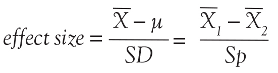
As the above equation shows, the effect size is expressed, in general, as a mean difference divided by a standard deviation. In the first case, the numerator represents the difference between the sample mean and the assumed population mean. In the denominator, SD is the standard deviation of the sample (used to estimate the standard deviation of the population). In the second case, the numerator represents the difference between the mean values of 2 samples and the denominator is the pooled standard deviation of the 2 samples.
In order to understand the issues involved with selecting sample size, we need to first understand the types of errors that can be made in any type of decision. Suppose our research goal is to make a decision about whether a new treatment results in a clinical difference (improvement). The results of our statistical test are dichotomous—we decide either yes there is a significant difference or no there isn’t. The truth, which we may never know, is that in reality, the difference exists or it doesn’t.

As Figure 7 shows, the result of our decision making is that there are 2 ways to be right and 2 ways to be wrong. If we decide there is a difference (eg, our statistical tests yields P ≤ .05) but in realty there is not a difference, then we make what is called a type I error. On the other hand, if we conclude that there is not a difference (ie, our statistical test yields P > .05) but in reality there is a difference that we did not detect, then we have made a type II error.

The associated math is shown in Figure 8. The probability of making a type I error is called alpha. By convention in medicine, we set our rejection criterion to alpha = 0.05. In other words, we would reject the null hypothesis (that there is no difference) anytime our statistical test yields a P value less than alpha. The probability of making a type II error is called beta. For historical reasons, the probability of not making a type II error is called the statistical power of the test and is equal to 1 minus beta. Power is affected by sample size: the larger the sample the larger the power. Most researchers, by convention, keep the sample size large enough to keep power above 0.80.

Figure 9 is a nomogram that brings all these ideas together. The red line shows that for your study, given the desired effect size (0.8), if you collected samples from the 30 patients you planned on then the power would be unacceptable at 0.60, indicating a high probability of a false negative decision if the P value comes out greater than .50. The solution is to increase the sample size to about 50 (or more), as indicated by the blue line. From this nomogram we can generalize to say that when you want to detect a small effect with data that have high variability, you need a large sample size to provide acceptable power.
The text below is an example of a power analysis presented in the methods section of a published study.20 Note that the authors give their reasoning for the sample size they selected. This kind of explanation may inform your study design. But what if you don’t know the variability of the data you want to collect? In that case, you need to collect some pilot data and calculate from that an appropriate sample size for a subsequent study.
A prospective power calculation indicated that a sample size of 25 per group was required to achieve 80% power based on an effect size of probability of 0.24 that an observation in the PRVCa group is less than an observation in the ASV group using the Mann-Whitney tests, an alpha of 0.05 (two-tailed) and a 20% dropout.
JUDGING FEASIBILITY
Once you have a draft of your study design, including the estimated sample size, it is time to judge the overall feasibility of the study before committing to it.

Every study has associated costs. Those costs and the sources of funding must be identified. Don’t forget costs for consultants, particularly if you need statistical consultation.
Finally, consider your level of experience. If you are contemplating your first study, a human clinical trial might not be the best choice, given the complexity of such a project. Studies such as a meta-analysis or mathematical simulation require special training beyond basic research procedures, and should be avoided.
- Tobin MJ. Mentoring: seven roles and some specifics. Am J Respir Crit Care Med 2004; 170:114–117.
- Chatburn RL. Advancing beyond the average: the importance of mentoring in professional achievement. Respir Care 2004; 49:304–308.
- Beveridge WIB. The Art of Scientific Investigation. New York, NY: WW Norton & Company; 1950.
- Chatburn RL, Mireles-Cabodevila E, Sasidhar M. Tidal volume measurement error in pressure control modes of mechanical ventilation: a model study. Comput Biol Med 2016; 75:235–242.
- Mireles-Cabodevila E, Chatburn RL. Work of breathing in adaptive pressure control continuous mandatory ventilation. Respir Care 2009; 54:1467–1472.
- Chatburn RL, Ford RM. Procedure to normalize data for benchmarking. Respir Care 2006; 51:145–157.
- Bou-Khalil P, Zeineldine S, Chatburn R, et al. Prediction of inspired oxygen fraction for targeted arterial oxygen tension following open heart surgery in non-smoking and smoking patients. J Clin Monit Comput 2016. https://doi.org/10.1007/s10877-016-9941-6.
- Mireles-Cabodevila E, Diaz-Guzman E, Arroliga AC, Chatburn RL. Human versus computer controlled selection of ventilator settings: an evaluation of adaptive support ventilation and mid-frequency ventilation. Crit Care Res Pract 2012; 2012:204314.
- Chatburn RL. How to find the best evidence. Respir Care 2009; 54:1360–1365.
- Durbin CG Jr. How to read a scientific research paper. Respir Care 2009; 54:1366–1371.
- Pierson DJ. How to read a case report (or teaching case of the month). Respir Care 2009; 54:1372–1378.
- Callcut RA, Branson RD. How to read a review paper. Respir Care 2009; 54:1379–1385.
- Eresuma E, Lake E. How do I find the evidence? Find your librarian—stat! Orthop Nurs 2016; 35:421–423.
- Janke R, Rush KL. The academic librarian as co-investigator on an interprofessional primary research team: a case study. Health Info Libr J 2014; 31:116–122.
- Motulsky H. Essential Biostatistics: A Nonmathematical Approach. New York, NY: Oxford University Press; 2016.
- Chatburn RL. Handbook for Health Care Research. 2nd ed. Sudbury, MA: Jones and Bartlett Publishers; 2011.
- Lang TA, Secic M. How to Report Statistics in Medicine. 2nd ed. Philadelphia, PA: American College of Physicians; 2006.
- Prescott RJ, Civil I. Lies, damn lies and statistics: errors and omission in papers submitted to INJURY 2010–2012. Injury 2013; 44:6–11.
- Fantoni DT, Ida KK, Lopes TF, Otsuki DA, Auler JO Jr, Ambrosio AM. A comparison of the cardiopulmonary effects of pressure controlled ventilation and volume controlled ventilation in healthy anesthetized dogs. J Vet Emerg Crit Care (San Antonio) 2016; 26:524–530.
- Gruber PC, Gomersall CD, Leung P, et al. Randomized controlled trial comparing adaptive-support ventilation with pressure-regulated volume-controlled ventilation with automode in weaning patients after cardiac surgery. Anesthesiology 2008; 109:81–87.
INTRODUCTION
Basic research skills are not acquired from medical school but from a mentor.1,2 A mentor with experience in study design and technical writing can make a real difference in your career. Most good mentors have more ideas for studies than they have time for research, so they are willing to share and guide your course. Your daily clinical experience provides a wealth of ideas in the form of “why do we do it this way” or “what is the evidence for” or “how can we improve outcomes or cut cost?” Of course, just about every study you read in a medical journal has suggestions for further research in the discussion section. Finally, keep in mind that the creation of study ideas and in particular, hypotheses, is a mysterious process, as this quote indicates: “It is not possible, deliberately, to create ideas or to control their creation. What we can do deliberately is to prepare our minds.” 3 Remember that chance favors the prepared mind.
DEVELOPING THE STUDY IDEA
Often, the most difficult task for someone new to research is developing a practical study idea. This section will explain a detailed process for creating a formal research protocol. We will focus on two common sticking points: (1) finding a good idea, and (2) developing a good idea into a problem statement.
Novice researchers with little experience, no mentors, and short time frames are encouraged not to take on a clinical human study as the principle investigator. Instead, device evaluations are a low-cost, time-efficient alternative. Human studies in the form of a survey are also possible and are often exempt from full Institutional Review Board (IRB) review. Many human-like conditions can be simulated, as was done, for example, in the study of patient-ventilator synchrony.4,5 And if you have the aptitude, whole studies can be based on mathematical models and predictions, particularly with the vast array of computer tools now available.6,7 And don’t forget studies based on surveys.8
A structured approach
A formal research protocol is required for any human research. However, it is also recommended for all but the simplest investigations. Most of the new researchers I have mentored take a rather lax approach to developing the protocol, and most IRBs are more interested in protecting human rights than validating the study design. As a result, much time is wasted and sometimes an entire study has to be abandoned due to poor planning. Figure 1 illustrates a structured approach that helps to ensure success. It shows a 3-step, iterative process.
The first step is a process of expanding the scope of the project, primarily through literature review. Along the way you learn (or invent) appropriate terminology and become familiar with the current state of the research art on a broad topic. For example, let’s suppose you were interested in the factors that affect the duration of mechanical ventilation. The literature review might include topics such as weaning and patient-ventilator synchrony as well as ventilator-associated pneumonia. During this process, you might discover that the topic of synchrony is currently generating a lot of interest in the literature and generating a lot of questions or confusion. You then focus on expanding your knowledge in this area.
In the second step, you might develop a theoretical framework for understanding patient-ventilator synchrony that could include a mathematical model and, perhaps, an idea to include simulation to study the problem.
In the third step, you need to narrow the scope of the study to a manageable level that includes identifying measurable outcome variables, creating testable hypotheses, considering experimental designs, and evaluating the overall feasibility of the study. At this point, you may discover that you cannot measure the specific outcome variables indicated by your theoretical framework. In that case, you need to create a new framework for supporting your research. Alternatively, you may find that it is not possible to conduct the study you envision given your resources. In that case, it is back to step 1.
Eventually, this process will result in a well-planned research protocol that is ready for review. Keep in mind that many times a protocol needs to be refined after some initial experiments are conducted. For human studies, any changes to the protocol must be approved by the IRB.
The problem statement rubric
The most common problem I have seen novices struggle with is creating a meaningful problem statement and hypothesis. This is crucial because the problem statement sets the stage for the methods, the methods yield the results, and the results are analyzed in light of the original problem statement and hypotheses. To get past any writer’s block, I recommend that you start by just describing what you see happening and why you think it is important. For example, you might say, “Patients with acute lung injury often seem to be fighting the ventilator.” This is important because patient-ventilator asynchrony may lead to increased sedation levels and prolonged intensive care unit stays. Now you can more easily envision a specific purpose and testable hypothesis. For example, you could state that the purpose of this study is to determine the baseline rates of different kinds of patient-ventilator synchrony problems. The hypothesis is that the rate of dyssynchrony is correlated with duration of mechanical ventilation.
Here is an actual example of how a problem statement evolved from a vague notion to a testable hypothesis.
Original: The purpose of this study is to determine whether measures of ineffective cough in patients with stroke recently liberated from mechanical ventilation correlate with risk of extubation failure and reintubation.
Final: The purpose of this study is to test the hypothesis that use of CoughAssist device in the immediate post-extubation period by stroke patients reduces the rate of extubation failure and pneumonia.
The original statement is a run-on sentence that is vague and hard to follow. Once the actual treatment and outcome measures are in focus, then a clear hypothesis statement can be made. Notice that the hypothesis should be clear enough that the reader can anticipate the actual experimental measures and procedures to be described in the methods section of the protocol.
Here is another example:
Original: The purpose of this study is to evaluate a device that allows continuous electronic cuff pressure control.
Final: The purpose of this study is to test the hypothesis that the Pressure Eyes electronic cuff monitor will maintain constant endotracheal tube cuff pressures better than manual cuff inflation during mechanical ventilation.
The problem with the original statement is that “to evaluate” is vague. The final statement makes the outcome variable explicit and suggests what the experimental procedure will be.
This is a final example:
Original: Following cardiac/respiratory arrest, many patients are profoundly acidotic. Ventilator settings based on initial arterial blood gases may result in inappropriate hyperventilation when follow-up is delayed. The purpose of this study is to establish the frequency of this occurrence at a large academic institution and the feasibility of a quality improvement project.
Final: The primary purpose of this study is to evaluate the frequency of hyperventilation occurring post-arrest during the first 24 hours. A secondary purpose is to determine if this hyperventilation is associated with an initial diagnosis of acidosis.
Note that the original statement follows the rubric of telling us what is observed and why it is important. However, the actual problem statement derived from the observation is vague: what is “this occurrence” and is the study really to establish any kind of feasibility? The purpose is simply to evaluate the frequency of hyperventilation and determine if the condition is associated with acidosis.
EXAMPLES OF RESEARCH PROJECTS BY FELLOWS
The following are examples of well-written statements of study purpose from actual studies conducted by our fellows.
Device evaluation
Defining “Flow Starvation” in volume control mechanical ventilation.
- The purpose of this study is to evaluate the relationship between the patient and ventilator inspiratory work of breathing to define the term “Flow Starvation.”
Auto-positive end expiratory pressure (auto-PEEP) during airway pressure release ventilation varies with the ventilator model.
- The purpose of this study was to compare auto-PEEP levels, peak expiratory flows, and flow decay profiles among 4 common intensive care ventilators.
Patient study
Diaphragmatic electrical activity and extubation outcomes in newborn infants: an observational study.
- The purpose of this study is to describe the electrical activity of the diaphragm before, during, and after extubation in a mixed-age cohort of preterm infants.
Comparison of predicted and measured carbon dioxide production for monitoring dead space fraction during mechanical ventilation.
- The purpose of this pilot study was to compare dead space with tidal volume ratios calculated from estimated and measured values for carbon dioxide production.
Practice evaluation
Incidence of asynchronies during invasive mechanical ventilation in a medical intensive care unit.
- The purpose of this study is to conduct a pilot investigation to determine the baseline incidence of various forms of patient-ventilator dyssynchrony during invasive mechanical ventilation.
Simulation training results in improved knowledge about intubation policies and procedures.
- The purpose of this study was to develop and test a simulation-based rapid-sequence intubation curriculum for fellows in pulmonary and critical care training.
HOW TO SEARCH THE LITERATURE
After creating a problem statement, the next step in planning research is to search the literature. The 10th issue of Respiratory Care journal in 2009 was devoted to research. Here are the articles in that issue related to the literature search:
- How to find the best evidence (search internet)9
- How to read a scientific research paper10
- How to read a case report (or teaching case of the month)11
- How to read a review paper.12
I recommend that you read these papers.
Literature search resources
My best advice is to befriend your local librarian.13 These people seldom get the recognition they deserve as experts at finding information and even as co-investigators.14 In addition to personal help, some libraries offer training sessions on various useful skills.
PubMed
The Internet resource I use most often is PubMed (www.ncbi.nlm.nih.gov/pubmed). It offers free access to MEDLINE, which is the National Library of Medicine’s database of citations and abstracts in the fields of medicine, nursing, dentistry, veterinary medicine, health care systems, and preclinical sciences. There are links to full-text articles and other resources. The website provides a clinical queries search filters page as well as a special queries page. Using a feature called “My NCBI,” you can have automatic e-mailing of search updates and save records and filters for search results. Access the PubMed Quick Start Guide for frequently asked questions and tutorials.
SearchMedica.com
The SearchMedica website (www.searchmedica.co.uk) is free and intended for medical professionals. It provides answers for clinical questions. Searches return articles, abstracts, and recommended medical websites.
Synthetic databases
There is a class of websites called synthetic databases, which are essentially prefiltered records for particular topics. However, these sites are usually subscription-based, and the cost is relatively high. You should check with your medical library to get access. Their advantage is that often they provide the best evidence without extensive searches of standard, bibliographic databases. Examples include the Cochrane Database of Systematic Reviews (www.cochrane.org/evidence), the National Guideline Clearinghouse (www.guideline.gov), and UpToDate (www.uptodate.com). UpToDate claims to be the largest clinical community in the world dedicated to synthesized knowledge for clinicians and patients. It features the work of more than 6,000 expert clinician authors/reviewers on more than 10,000 topics in 23 medical specialties. The site offers graded recommendations based on the best medical evidence.
Portals
Portals are web pages that act as a starting point for using the web or web-based services. One popular example is ClinicalKey (www.clinicalkey.com/info), formerly called MD Consult, which offers books, journals, patient education materials, and images. Another popular portal is Ovid (ovid.com), offering books, journals, evidence-based medicine databases, and CINAHL (Cumulative Index to Nursing and Allied Health Literature).
Electronic journals
Many medical journals now have online databases of current and archived issues. Such sites may require membership to access the databases, so again, check with your medical library. Popular examples in pulmonary and critical care medicine include the following:
- American Journal of Respiratory and Critical Care Medicine (www.atsjournals.org/journal/ajrccm)
- The New England Journal of Medicine (www.nejm.org)
- Chest (journal.publications.chestnet.org)
- Respiratory Care (rc.rcjournal.com)
Electronic books
Amazon.com is a great database search engine for books on specific topics. It even finds out-of-print books. And you don’t have to buy the books, because now you can rent them. Sometimes, I find what I wanted by using the “Look Inside” feature for some books. Note that you can look for books at PubMed. Just change the search box from PubMed to Books on the PubMed home page. Of course, Google also has a book search feature. A great (subscription) resource for medical and technical books is Safari (https://www.safaribooksonline.com). Once again, your library may have a subscription.
General Internet resources
You probably already know about Google Scholar (scholar.google.com) and Wikipedia.com. Because of its open source nature, you should use Wikipedia with caution. However, I have found it to be a very good first step in finding technical information, particularly about mathematics, physics, and statistics.
Using reference management software
One of the most important things you can do to make your research life easier is to use some sort of reference management software. As described in Wikipedia, “Reference management software, citation management software or personal bibliographic management software is software for scholars and authors to use for recording and using bibliographic citations (references). Once a citation has been recorded, it can be used time and again in generating bibliographies, such as lists of references in scholarly books, articles, and essays.” I was late in adopting this technology, but now I am a firm believer. Most Internet reference sources offer the ability to download citations to your reference management software. Downloading automatically places the citation into a searchable database on your computer with backup to the Internet. In addition, you can get the reference manager software to find a PDF version of the manuscript and store it with the citation on your computer (and/or in the Cloud) automatically.
But the most powerful feature of such software is its ability to add or subtract and rearrange the order of references in your manuscripts as you are writing, using seamless integration with Microsoft Word. The references can be automatically formatted using just about any journal’s style. This is a great time saver for resubmitting manuscripts to different journals. If you are still numbering references by hand (God forbid) or even using the Insert Endnote feature in Word (deficient when using multiple occurrences of the same reference), your life will be much easier if you take the time to start using reference management software.
The most popular commercial software is probably EndNote (endnote.com). A really good free software system with about the same functionality as Zotero (zotero.com). Search for “comparison of reference management software” in Wikipedia. You can find tutorials on software packages in YouTube.
STUDY DESIGN
When designing the experiment, note that there are many different approaches, each with their advantages and disadvantages. A full treatment of this topic is beyond the scope of this article. Suffice it to say that pre-experimental designs (Figure 2) are considered to generate weak evidence. But they are quick and easy and might be appropriate for pilot studies.
Quasi-experimental designs (Figure 3) generate a higher level of evidence. Such a design might be appropriate when you are stuck with collecting a convenience sample, rather than being able to use a full randomized assignment of study subjects.
The fully randomized design (Figure 4) generates the highest level of evidence. This is because if the sample size is large enough, the unknown and uncontrollable sources of bias are evenly distributed between the study groups.
BASIC MEASUREMENT METHODS
If your research involves physical measurements, you need to be familiar with the devices considered to be the gold standards. In cardiopulmonary research, most measurements involve pressure volume, flow, and gas concentration. You need to know which devices are appropriate for static vs dynamic measurements of these variables. In addition, you need to understand issues related to systematic and random measurement errors and how these errors are managed through calibration and calibration verification. I recommend these two textbooks:
Principles and Practice of Intensive Care Monitoring 1st Edition by Martin J. Tobin MD.
- This book is out of print, but if you can find a used copy or one in a library, it describes just about every kind of physiologic measurement used in clinical medicine.
Medical Instrumentation: Application and Design 4th Edition by John G. Webster.
- This book is readily available and reasonably priced. It is a more technical book describing medical instrumentation and measurement principles. It is a standard textbook for biometrical engineers.
STATISTICS FOR THE UNINTERESTED
I know what you are thinking: I hate statistics. Look at the book Essential Biostatistics: A Nonmathematical Approach.15 It is a short, inexpensive paperback book that is easy to read. The author does a great job of explaining why we use statistics rather than getting bogged down explaining how we calculate them. After all, novice researchers usually seek the help of a professional statistician to do the heavy lifting.
My book, Handbook for Health Care Research,16 covers most of the statistical procedures you will encounter in medical research and gives examples of how to use a popular tactical software package called SigmaPlot. By the way, I strongly suggest that you consult a statistician early in your study design phase to avoid the disappointment of finding out later that your results are uninterpretable. For an in-depth treatment of the subject, I recommend How to Report Statistics in Medicine.17
Statistical bare essentials
To do research or even just to understand published research reports, you must have at least a minimal skill set. The necessary skills include understanding some basic terminology, if only to be able to communicate with a statistician consultant. Important terms include levels of measurement (nominal, ordinal, continuous), accuracy, precision, measures of central tendency (mean, median, mode), measures of variability (variance, standard deviation, coefficient of variation), and percentile. The first step in analyzing your results is usually to represent it graphically. That means you should be able to use a spreadsheet to make simple graphs (Figure 5).
You should also know the basics of inferential statistics (ie, hypothesis testing). For example, you need to know the difference between parametric and non-parametric tests. You should be able to explain correlation and regression and know when to use Chi-squared vs a Fisher exact test. You should know that when comparing two mean values, you typically use the Student’s t test (and know when to use paired vs unpaired versions of the test). When comparing more than 2 mean values, you use analysis of variance methods (ANOVA). You can teach yourself these concepts from a book,16 but even an introductory college level course on statistics will be immensely helpful. Most statistics textbooks provide some sort of map to guide your selection of the appropriate statistical test (Figure 6), and there are good articles in medical journals.
You can learn a lot simply by reading the Methods section of research articles. Authors will often describe the statistical tests used and why they were used. But be aware that a certain percentage of papers get published with the wrong statistics.18
One of the underlying assumptions of most parametric statistical methods is that the data may be adequately described by a normal or Gaussian distribution. This assumption needs to be verified before selecting a statistical test. The common test for data normality is the Kolmogorov-Smirnov test. The following text from a methods section describes 2 very common procedures—the Student’s t test for comparing 2 mean values and the one-way ANOVA for comparing more than 2 mean values.19
“Normal distribution of data was verified using the Kolmogorov-Smirnov test. Body weights between groups were compared using one-way ANOVA for repeated measures to investigate temporal differences. At each time point, all data were analyzed using one-way ANOVA to compare PCV and VCV groups. Tukey’s post hoc analyses were performed when significant time effects were detected within groups, and Student’s t test was used to investigate differences between groups. Data were analyzed using commercial software and values were presented as mean ± SD. A P value < .05 was considered statistically significant.”
Estimating sample size and power analysis
One very important consideration in any study is the required number of study subjects for meaningful statistical conclusions. In other words, how big should the sample size be? Sample size is important because it affects the feasibility of the study and the reliability of the conclusions in terms of statistical power. The necessary sample size depends on 2 basic factors. One factor is the variability of the data (often expressed as the standard deviation). The other factor is the effect size, meaning, for example, how big of a difference between mean values you want to detect. In general, the bigger the variability and the smaller the difference, the bigger the sample size required.
As the above equation shows, the effect size is expressed, in general, as a mean difference divided by a standard deviation. In the first case, the numerator represents the difference between the sample mean and the assumed population mean. In the denominator, SD is the standard deviation of the sample (used to estimate the standard deviation of the population). In the second case, the numerator represents the difference between the mean values of 2 samples and the denominator is the pooled standard deviation of the 2 samples.
In order to understand the issues involved with selecting sample size, we need to first understand the types of errors that can be made in any type of decision. Suppose our research goal is to make a decision about whether a new treatment results in a clinical difference (improvement). The results of our statistical test are dichotomous—we decide either yes there is a significant difference or no there isn’t. The truth, which we may never know, is that in reality, the difference exists or it doesn’t.
As Figure 7 shows, the result of our decision making is that there are 2 ways to be right and 2 ways to be wrong. If we decide there is a difference (eg, our statistical tests yields P ≤ .05) but in realty there is not a difference, then we make what is called a type I error. On the other hand, if we conclude that there is not a difference (ie, our statistical test yields P > .05) but in reality there is a difference that we did not detect, then we have made a type II error.
The associated math is shown in Figure 8. The probability of making a type I error is called alpha. By convention in medicine, we set our rejection criterion to alpha = 0.05. In other words, we would reject the null hypothesis (that there is no difference) anytime our statistical test yields a P value less than alpha. The probability of making a type II error is called beta. For historical reasons, the probability of not making a type II error is called the statistical power of the test and is equal to 1 minus beta. Power is affected by sample size: the larger the sample the larger the power. Most researchers, by convention, keep the sample size large enough to keep power above 0.80.
Figure 9 is a nomogram that brings all these ideas together. The red line shows that for your study, given the desired effect size (0.8), if you collected samples from the 30 patients you planned on then the power would be unacceptable at 0.60, indicating a high probability of a false negative decision if the P value comes out greater than .50. The solution is to increase the sample size to about 50 (or more), as indicated by the blue line. From this nomogram we can generalize to say that when you want to detect a small effect with data that have high variability, you need a large sample size to provide acceptable power.
The text below is an example of a power analysis presented in the methods section of a published study.20 Note that the authors give their reasoning for the sample size they selected. This kind of explanation may inform your study design. But what if you don’t know the variability of the data you want to collect? In that case, you need to collect some pilot data and calculate from that an appropriate sample size for a subsequent study.
A prospective power calculation indicated that a sample size of 25 per group was required to achieve 80% power based on an effect size of probability of 0.24 that an observation in the PRVCa group is less than an observation in the ASV group using the Mann-Whitney tests, an alpha of 0.05 (two-tailed) and a 20% dropout.
JUDGING FEASIBILITY
Once you have a draft of your study design, including the estimated sample size, it is time to judge the overall feasibility of the study before committing to it.
Every study has associated costs. Those costs and the sources of funding must be identified. Don’t forget costs for consultants, particularly if you need statistical consultation.
Finally, consider your level of experience. If you are contemplating your first study, a human clinical trial might not be the best choice, given the complexity of such a project. Studies such as a meta-analysis or mathematical simulation require special training beyond basic research procedures, and should be avoided.
- Tobin MJ. Mentoring: seven roles and some specifics. Am J Respir Crit Care Med 2004; 170:114–117.
- Chatburn RL. Advancing beyond the average: the importance of mentoring in professional achievement. Respir Care 2004; 49:304–308.
- Beveridge WIB. The Art of Scientific Investigation. New York, NY: WW Norton & Company; 1950.
- Chatburn RL, Mireles-Cabodevila E, Sasidhar M. Tidal volume measurement error in pressure control modes of mechanical ventilation: a model study. Comput Biol Med 2016; 75:235–242.
- Mireles-Cabodevila E, Chatburn RL. Work of breathing in adaptive pressure control continuous mandatory ventilation. Respir Care 2009; 54:1467–1472.
- Chatburn RL, Ford RM. Procedure to normalize data for benchmarking. Respir Care 2006; 51:145–157.
- Bou-Khalil P, Zeineldine S, Chatburn R, et al. Prediction of inspired oxygen fraction for targeted arterial oxygen tension following open heart surgery in non-smoking and smoking patients. J Clin Monit Comput 2016. https://doi.org/10.1007/s10877-016-9941-6.
- Mireles-Cabodevila E, Diaz-Guzman E, Arroliga AC, Chatburn RL. Human versus computer controlled selection of ventilator settings: an evaluation of adaptive support ventilation and mid-frequency ventilation. Crit Care Res Pract 2012; 2012:204314.
- Chatburn RL. How to find the best evidence. Respir Care 2009; 54:1360–1365.
- Durbin CG Jr. How to read a scientific research paper. Respir Care 2009; 54:1366–1371.
- Pierson DJ. How to read a case report (or teaching case of the month). Respir Care 2009; 54:1372–1378.
- Callcut RA, Branson RD. How to read a review paper. Respir Care 2009; 54:1379–1385.
- Eresuma E, Lake E. How do I find the evidence? Find your librarian—stat! Orthop Nurs 2016; 35:421–423.
- Janke R, Rush KL. The academic librarian as co-investigator on an interprofessional primary research team: a case study. Health Info Libr J 2014; 31:116–122.
- Motulsky H. Essential Biostatistics: A Nonmathematical Approach. New York, NY: Oxford University Press; 2016.
- Chatburn RL. Handbook for Health Care Research. 2nd ed. Sudbury, MA: Jones and Bartlett Publishers; 2011.
- Lang TA, Secic M. How to Report Statistics in Medicine. 2nd ed. Philadelphia, PA: American College of Physicians; 2006.
- Prescott RJ, Civil I. Lies, damn lies and statistics: errors and omission in papers submitted to INJURY 2010–2012. Injury 2013; 44:6–11.
- Fantoni DT, Ida KK, Lopes TF, Otsuki DA, Auler JO Jr, Ambrosio AM. A comparison of the cardiopulmonary effects of pressure controlled ventilation and volume controlled ventilation in healthy anesthetized dogs. J Vet Emerg Crit Care (San Antonio) 2016; 26:524–530.
- Gruber PC, Gomersall CD, Leung P, et al. Randomized controlled trial comparing adaptive-support ventilation with pressure-regulated volume-controlled ventilation with automode in weaning patients after cardiac surgery. Anesthesiology 2008; 109:81–87.

Chi-square and Fisher’s exact tests
This article aims to introduce the statistical methodology behind chi-square and Fisher’s exact tests, which are commonly used in medical research to assess associations between categorical variables. This discussion will use data from a study by Mrozek1 in patients with acute respiratory distress syndrome (ARDS). This was a multicenter, prospective, observational study: multicenter because it included data from 10 intensive care units, prospective because the study collected the data moving forward in time, and observational because the study investigators did not have control over the group assignments but rather used the naturally occurring groups. The study objective was to characterize focal and nonfocal patterns of lung computed tomography (CT)-based imaging with plasma markers of lung injury.
The primary grouping variable was type of ARDS (focal vs nonfocal) as determined by CT scans and other lung imaging tools. In this study, there were 32 (27%) patients with focal ARDS and 87 (73%) patients with nonfocal ARDS. What will be important, however, is classifying the type of variables because this determines the type of analyses performed. Type of ARDS is a categorical variable with 2 levels.
The primary study endpoint was plasma levels of the soluble form of the receptor for advanced glycation end product. There were also a number of secondary study endpoints that can be grouped as either patient outcomes or biomarkers. Patient outcomes included the duration of mechanical ventilation and both 28- and 90-day mortality. Levels of other biomarkers included surfactant protein D, soluble intercellular adhesion molecule-1, and plasminogen activator inhibitor-1.
This article focused on the secondary outcome of 90-day mortality beginning at disease onset. Again, we are interested in classifying this variable, which is categorical with 2 levels (yes vs no). So the scenario is that we want to assess the relationship between the type of ARDS (focal vs nonfocal) and 90-day mortality (yes vs no). In its most basic form, this scenario is an investigation into the association among 2 categorical variables.
.")
When there are 2 categorical variables, the data can be arranged in what is called a contingency table (Figure 1). Because both variables are binary (2 levels), it is called a 2 × 2 table. However, a contingency table can be generated for 2 categorical variables with any number of levels—in that case, it is called an r ×c table, where r is the number of levels for the row variable and c is the number of levels for the column variable. The actual raw counts or frequencies are recorded inside the table cells. The cell counts are often referred to as observed counts and thus the notation (Oij) is used. The subscript i identifies the specific level of the row variable, and in this example it can equal 1 or 2 since the row variable is binary. Similarly, the subscript j identifies the specific level of the column variable and in this example it can equal 1 or 2 since the column variable is binary. Therefore, O11 represents the number of patients who have the row variable = level 1 and the column variable = level 1.
In addition to the row and column variable cells, there are also the margin totals. These totals are either the row margin total (summing across the row) or the column margin total (summing down the column). For example, n1+ is the sum of the row where the row variable equal 1 (O11 + O12 = n1+). Finally, at the very bottom right corner is the grand total, which equals the sample size.
The goal is to test whether or not these 2 categorical variables are associated with each other. The null hypothesis (Ho) is that there is no association between these 2 categorical variables and the alternative hypotheses (Ha) is that there is an association between these 2 categorical variables.
The next step is to translate the generic form of the hypotheses into hypotheses that are specific to the research question. In this case, the null hypothesis is that mortality is not associated with lung morphology and the alternative hypothesis is that mortality is associated with lung morphology.
The contingency table cells can be populated with the numbers found in the article. It has our outcome of focus—mortality at day 90—both the count and the percent. The results are broken down by type of ARDS (focal vs nonfocal) as follows:
- Focal ARDS = 6 patients (21.4%)
- Nonfocal ARDS = 35 patients (45.5%).

First, the row variable is lung morphology, and it has two levels (focal vs nonfocal). Next, the column variable is 90-day mortality and it has 2 levels (yes vs no). Finally, the table must be populated, but be careful not to assume that there are no missing data. Begin with the cell counts: there were 6 focal ARDS patients and 35 nonfocal ARDS patients who died within 90 days. These two numbers populate the first column and result in a column total of 41. Next, use the reported percentages to calculate the row totals. Six is 21.4% of 28, so the first row total is 28. Thirty-five is 45.5% of 77, so the second row total is 77. If there are 28 patients with focal ARDS and 77 with nonfocal ARDS, then the grand total is 28 + 77 = 105. The remaining values can be obtained by subtraction. If there are 105 total patients and 41 die within 90 days, then 105 − 41 = 64 patients who do not die within 90 days and this is the second column total. Similarly, if there are 28 focal ARDS patients and 6 die within 90 days, then 28 − 6 = 22 patients who do not die within 90 days. Lastly, if there are 77 nonfocal ARDS patients and 35 die within 90 days, then 77 − 35 = 42 patients who do not die within 90 days. Now the contingency table is complete.
Once the contingency table is built, the question becomes, “Is lung morphology associated with 90-day mortality?” To answer that question, we need to know how many patients one would expect in each table cell if the null hypothesis of no association is true. When conducting a hypothesis test, one always assumes that the null hypothesis is true and then gathers data to see how well the data aligns with that assumption.
So one must calculate how many patients to expect in each of these cells if lung morphology is not associated with 90-day mortality. One way to address this question is to ask these 2 questions:
(1) Overall, what proportion of patients die by day 90? Looking at the constructed contingency table, that answer would be 39%. This was calculated by taking the total number of patients who died by day 90 and dividing it by the total number of patients, 41/105 = 39%. This gives the overall proportion, based on the data, who would die by day 90.
(2) How many of the focal ARDS patients would be expected to die by day 90? Now it is not overall, but rather we are limiting the question to the focal ARDS group. To obtain the answer, multiply the overall proportion of patients who die by day 90 by how many focal ARDS patients are in the study. Essentially, take the answer from the previous question and multiply it by the total number of focal ARDS, which is 28. The result is (41/105) × 28 = 10.9. Thus, if there is no association among long morphology and 90-day mortality, one would expect 10.9 focal ARDS patients to die by day 90.
Now 10.9 is a very specific answer for a specific contingency table, but the answer could be written in general terms. Basically, 3 numbers were used in calculating the solution: the row margin, the column margin, and the grand total. The general formula is the following:
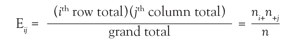
The notation Eij is used to represent the expected count assuming the null hypothesis of no association among the row and column variables is true. To calculate the expected count, take the ith row total times the jth column total and divide by the grand total.
In the lung morphology and mortality example, what is the expected number of deaths within 90 days among the nonfocal ARDS patients? This is the second row and the first column (E21). Applying the formula, one multiplies the total for the second row by the total for the first column and then divides by the grand total, (77 × 41)/105 = 30.1. This calculation is repeated for each of the 4 cells.
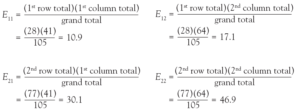
Because we now know the observed cell count and the expected cell count (under the null hypothesis), we can compare the observed and expected counts to see how well the data aligns with the null hypothesis. This is what the chi-square test does, and the test statistic is calculated as follows:

The sigma (Σ) means addition, so the calculation is performed on each individual cell in the contingency table and then the results are summed. A 2 × 2 table has 4 cells and thus 4 numbers will be summed. For each cell, the formula compares the observed to the expected. Basically, it computes how similar they are (that is the O minus E part). Because the differences will be positive for some cells and negative for others, the differences are squared to avoid cancellation when you add them. Finally, each squared difference is divided by the expected count to standardize the calculation.
Intuitively, if the observed counts (Oij) are similar to the expected counts under the null hypothesis (Eij), then these 2 numbers will be very close to each other. When taking the difference between them or subtracting them, the result is a small number. When squaring a small number, one obtains a really small number. And adding up a bunch of really small numbers results in a small number. So the test statistic is going to be small. That means that the resulting P value is going to be large. What is a P value? Think of it as an index of compatibility. How compatible is the data with the null hypothesis? Here, you get a large index of compatibility. That means that the data aligns nicely with the null hypothesis and one fails to reject the null.
Now, think about the alternative scenario. If the observed counts (Oij) are wildly different from the expected counts under the null hypothesis (Eij), then these 2 numbers will be quite different. When taking the difference between them or subtracting them, the result is a big number. When squaring a big number, one obtains a really big number, and adding up a bunch of really big numbers results in a large number. So the test statistic is going to be large. That means that the resulting P value is going to be small. And if you think of a P value as an index of compatibility, the data and the null hypothesis are not very compatible. That means that the data does not align nicely with the null hypothesis and one rejects the null. This is the general idea of the chi-square test. It assesses how compatible the data is with the null hypothesis that the 2 categorical variables are not associated.
To obtain the actual P value, the distribution of the test statistic (under the null hypothesis) is used to calculate the area under the curve for values equal to the test statistic or more extreme. The described test statistic has an approximate chi-square distribution with (r − 1)(c − 1) degree of freedom. Recall that r is the number of levels of the row variable and c is the number of levels of the column variable. Our example is a 2 × 2 table, so the test statistic has an approximate chi-square distribution with (2 − 1)(2 − 1) = 1 degree of freedom.
Now that the chi-square test has been fully described, the assumptions for the test must be discussed. It is important to know when you should or should not perform this test. The chi-square test assumes that observations are independent. This means that the outcome for one observation is not associated with the outcome of any other observation. This principle can be violated when multiple measurements are taken over time or when multiple measurements are taken from one patient.
Another assumption is that the chi-square large sample approximation just described is appropriate. In other words, no more than 20% of the expected counts (Eij) are less than 5. For a 2 × 2 table, how many cells do you have? Four. So if even one of those 4 happens to have an expected count less than 5, this assumption is violated. For a 2 × 2 table, none of the expected counts can be less than 5.
Returning to the lung morphology and mortality example, were the assumptions met? The data consist of 105 unique patients. Thus, we can assume that they are independent. The minimum expected count was 10.9, which is not less than 5. Therefore, the assumptions for the chi-square test are met. Next, the test statistic is calculated using the observed and expected counts. For each cell, subtract the expected count from the observed count, square it, and divide by the expected count. Then, add the 4 resulting numbers to obtain the test statistic of 4.92.
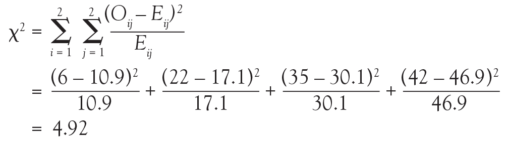

Finally, compute the area under the chi-square distribution with 1 degree of freedom Χ2(1), at the test statistic and values more extreme. In this case, values more extreme are values greater than the test statistic. Here, the area under the curve to the right of 4.92 is .027 (Figure 3). This is the P value, which indicates that the data and the null hypothesis have very low compatibility. In this example, the area under the curve to the right of 4.92 is .027 (Figure 3). This is the P value, which indicates that the data and the null hypothesis have very low compatibility. Thus, the decision is to reject the null hypothesis. The conclusion is that lung morphology is associated with 90-day mortality (P = .027). To describe that association, one looks at the contingency table and finds a reduction in 90-day mortality with focal patterns compared to nonfocal patterns (21.4% vs 45.5%, respectively). The P value reported in the article is .026. Our hand calculation was .027, which is slightly off due to rounding. In summary, the scenario is an investigation into the association among 2 categorical variables, and, thus, a test to consider is the chi-square test, if assumptions are met.
In another example in the same study, the authors investigate whether any baseline characteristics are associated with lung morphology. For example, is neurology, specifically Parkinson disease (yes vs no), associated with lung morphology (focal vs nonfocal)? Again, the scenario is an investigation into the association between 2 categorical variables, so a chi-square test should be considered.

To start, build a contingency table arbitrarily placing lung morphology as the row variable and Parkinson disease as the column variable. Populate the contingency table based on the counts and percentages reported in the article (Figure 4). Next, check that the assumptions of the chi-square test are met. Are the observations independent? Again, because these are unique patients, we consider this assumption met. Since this is a 2 × 2 table, are all of the expected counts greater than 5? Calculations of the expected counts obtained the following: 1.1, 30.9, 2.9 and 84.1. Here, 2 of the 4 expected counts are less than 5. Therefore, methods that use large sample approximation, like the chi-squared test, may not be an appropriate choice.
Instead of using methodology that is an approximation, consider an exact test such as Fisher’s exact test. Again, refer to the contingency table where Fisher’s exact is going to calculate the exact probability (under the null hypothesis) of the observed data or results more extreme. This is the technical definition of a P value. It is, however, still quantifying how compatible the data are with the null hypothesis. The exact probability of a particular contingency table can be obtained using the hypergeometric distribution.
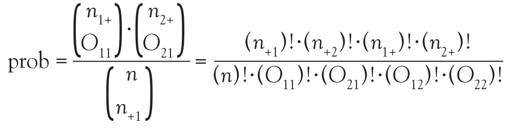
The symbols that resemble large parentheses are notations for a combinatorial. Because using combinatorials to calculate the probability is not user friendly, an equivalent version relies on factorials instead. Both techniques are presented above. Remember that the goal is to find the exact probability of the observed data or something more extreme.
The hypotheses are still testing whether these 2 categorical variables are associated with each other. In this particular example, we test if the proportion of patients with Parkinson disease is the same in the focal and nonfocal groups. Fisher’s exact test obtains its two-tailed P value by computing the probabilities associated with all possible tables that have the same row and column totals. Then, it identifies the alternative tables with a probability that is less than that of the observed table. Finally, it adds the probability of the observed table with the sum of the probabilities of each alternative table identified above, which results in the P value.

To explore each of those steps in detail, one must first enumerate how many tables can be built that all have the same row and column totals as the observed table. Figure 5 shows the 5 possible tables. Pick any one of the 5 2 × 2 tables; the margins are fixed. Each table has the same row totals, 32 focal and 87 nonfocal, and each table has the same column totals: 4 Parkinson and 115 non-Parkinson. Then, for each table, calculate the probability of that table. Figure 5 shows this calculation for the first 2 × 2 table, which happens to be the observed table. The probability of the table observed in the study is .2803. Such a calculation is performed on each of the other tables.
Next, one must identify the tables that have a probability smaller than the observed table. Here, we are looking for probabilities less than .2803. These are the tables deemed more extreme. Tables 3, 4, and 5 have probabilities less than .2803.
The final step is to sum the probability of the observed table and the more extreme tables (ie, those with probabilities < the observed table) (.2803 + .2337 + .0543 + .0045 = .5728). Thus, the resulting rounded P value is .57, which indicates a high level of compatibility between the data and the null hypothesis of no association. The decision is to fail to reject the null hypothesis and the conclusion is that the evidence does not support an association among lung morphology and Parkinson disease. In other words, there is insufficient evidence to claim that the proportion of Parkinson disease differs between the focal and nonfocal ARDS patients (0% vs 5%, P = .57). This matches the P value reported by Mrozek for this association.
The first objective of this article was to identify scenarios in which a chi-square or Fisher’s exact test should be considered. The general setting discussed was an investigation of the association between two categorical variables. Use of each test specifically depends on whether the assumptions have been met. Both of the examples used in our discussion happened to be binary, but that is not a restriction. Categorical variables can have more than 2 levels. All of the methods demonstrated for 2 × 2 tables can be generalized to r × c tables.
The second objective of this article was to recognize when test assumptions have been violated. For simplicity, most researchers adhere to the following: if ≤ 20% of expected cell counts are less than 5, then use the chi-square test; if > 20% of expected cell counts are less than 5, then use Fisher’s exact test. Both methods assume that the observations are independent. Could one use the exact test when the chi-square assumptions are met? Yes, but it is more computationally expensive as it uses all possible fixed margin tables and their probabilities. If the chi-square assumptions are met, then the sample size is typically larger and these calculations become numerous. Also, it does not have to be that large of a sample for the chi-square to be a good approximation and do it very quickly.
The final objective of this article was to test claims made regarding the association of 2 independent categorical variables. We included examples from the medical literature showing step-by-step calculations of both the large sample approximation (chi-square) and exact (Fisher’s) methodologies providing insight into how these tests are conducted as well as when they are appropriate.
- Mrozek S, Jabaudon M, Jaber S, et al. Elevated plasma levels of sRAGE are associated with nonfocal CT-based lung imaging in patients with ARDS. Chest 2016; 150:998–1007.
This article aims to introduce the statistical methodology behind chi-square and Fisher’s exact tests, which are commonly used in medical research to assess associations between categorical variables. This discussion will use data from a study by Mrozek1 in patients with acute respiratory distress syndrome (ARDS). This was a multicenter, prospective, observational study: multicenter because it included data from 10 intensive care units, prospective because the study collected the data moving forward in time, and observational because the study investigators did not have control over the group assignments but rather used the naturally occurring groups. The study objective was to characterize focal and nonfocal patterns of lung computed tomography (CT)-based imaging with plasma markers of lung injury.
The primary grouping variable was type of ARDS (focal vs nonfocal) as determined by CT scans and other lung imaging tools. In this study, there were 32 (27%) patients with focal ARDS and 87 (73%) patients with nonfocal ARDS. What will be important, however, is classifying the type of variables because this determines the type of analyses performed. Type of ARDS is a categorical variable with 2 levels.
The primary study endpoint was plasma levels of the soluble form of the receptor for advanced glycation end product. There were also a number of secondary study endpoints that can be grouped as either patient outcomes or biomarkers. Patient outcomes included the duration of mechanical ventilation and both 28- and 90-day mortality. Levels of other biomarkers included surfactant protein D, soluble intercellular adhesion molecule-1, and plasminogen activator inhibitor-1.
This article focused on the secondary outcome of 90-day mortality beginning at disease onset. Again, we are interested in classifying this variable, which is categorical with 2 levels (yes vs no). So the scenario is that we want to assess the relationship between the type of ARDS (focal vs nonfocal) and 90-day mortality (yes vs no). In its most basic form, this scenario is an investigation into the association among 2 categorical variables.
When there are 2 categorical variables, the data can be arranged in what is called a contingency table (Figure 1). Because both variables are binary (2 levels), it is called a 2 × 2 table. However, a contingency table can be generated for 2 categorical variables with any number of levels—in that case, it is called an r ×c table, where r is the number of levels for the row variable and c is the number of levels for the column variable. The actual raw counts or frequencies are recorded inside the table cells. The cell counts are often referred to as observed counts and thus the notation (Oij) is used. The subscript i identifies the specific level of the row variable, and in this example it can equal 1 or 2 since the row variable is binary. Similarly, the subscript j identifies the specific level of the column variable and in this example it can equal 1 or 2 since the column variable is binary. Therefore, O11 represents the number of patients who have the row variable = level 1 and the column variable = level 1.
In addition to the row and column variable cells, there are also the margin totals. These totals are either the row margin total (summing across the row) or the column margin total (summing down the column). For example, n1+ is the sum of the row where the row variable equal 1 (O11 + O12 = n1+). Finally, at the very bottom right corner is the grand total, which equals the sample size.
The goal is to test whether or not these 2 categorical variables are associated with each other. The null hypothesis (Ho) is that there is no association between these 2 categorical variables and the alternative hypotheses (Ha) is that there is an association between these 2 categorical variables.
The next step is to translate the generic form of the hypotheses into hypotheses that are specific to the research question. In this case, the null hypothesis is that mortality is not associated with lung morphology and the alternative hypothesis is that mortality is associated with lung morphology.
The contingency table cells can be populated with the numbers found in the article. It has our outcome of focus—mortality at day 90—both the count and the percent. The results are broken down by type of ARDS (focal vs nonfocal) as follows:
- Focal ARDS = 6 patients (21.4%)
- Nonfocal ARDS = 35 patients (45.5%).
First, the row variable is lung morphology, and it has two levels (focal vs nonfocal). Next, the column variable is 90-day mortality and it has 2 levels (yes vs no). Finally, the table must be populated, but be careful not to assume that there are no missing data. Begin with the cell counts: there were 6 focal ARDS patients and 35 nonfocal ARDS patients who died within 90 days. These two numbers populate the first column and result in a column total of 41. Next, use the reported percentages to calculate the row totals. Six is 21.4% of 28, so the first row total is 28. Thirty-five is 45.5% of 77, so the second row total is 77. If there are 28 patients with focal ARDS and 77 with nonfocal ARDS, then the grand total is 28 + 77 = 105. The remaining values can be obtained by subtraction. If there are 105 total patients and 41 die within 90 days, then 105 − 41 = 64 patients who do not die within 90 days and this is the second column total. Similarly, if there are 28 focal ARDS patients and 6 die within 90 days, then 28 − 6 = 22 patients who do not die within 90 days. Lastly, if there are 77 nonfocal ARDS patients and 35 die within 90 days, then 77 − 35 = 42 patients who do not die within 90 days. Now the contingency table is complete.
Once the contingency table is built, the question becomes, “Is lung morphology associated with 90-day mortality?” To answer that question, we need to know how many patients one would expect in each table cell if the null hypothesis of no association is true. When conducting a hypothesis test, one always assumes that the null hypothesis is true and then gathers data to see how well the data aligns with that assumption.
So one must calculate how many patients to expect in each of these cells if lung morphology is not associated with 90-day mortality. One way to address this question is to ask these 2 questions:
(1) Overall, what proportion of patients die by day 90? Looking at the constructed contingency table, that answer would be 39%. This was calculated by taking the total number of patients who died by day 90 and dividing it by the total number of patients, 41/105 = 39%. This gives the overall proportion, based on the data, who would die by day 90.
(2) How many of the focal ARDS patients would be expected to die by day 90? Now it is not overall, but rather we are limiting the question to the focal ARDS group. To obtain the answer, multiply the overall proportion of patients who die by day 90 by how many focal ARDS patients are in the study. Essentially, take the answer from the previous question and multiply it by the total number of focal ARDS, which is 28. The result is (41/105) × 28 = 10.9. Thus, if there is no association among long morphology and 90-day mortality, one would expect 10.9 focal ARDS patients to die by day 90.
Now 10.9 is a very specific answer for a specific contingency table, but the answer could be written in general terms. Basically, 3 numbers were used in calculating the solution: the row margin, the column margin, and the grand total. The general formula is the following:
The notation Eij is used to represent the expected count assuming the null hypothesis of no association among the row and column variables is true. To calculate the expected count, take the ith row total times the jth column total and divide by the grand total.
In the lung morphology and mortality example, what is the expected number of deaths within 90 days among the nonfocal ARDS patients? This is the second row and the first column (E21). Applying the formula, one multiplies the total for the second row by the total for the first column and then divides by the grand total, (77 × 41)/105 = 30.1. This calculation is repeated for each of the 4 cells.
Because we now know the observed cell count and the expected cell count (under the null hypothesis), we can compare the observed and expected counts to see how well the data aligns with the null hypothesis. This is what the chi-square test does, and the test statistic is calculated as follows:
The sigma (Σ) means addition, so the calculation is performed on each individual cell in the contingency table and then the results are summed. A 2 × 2 table has 4 cells and thus 4 numbers will be summed. For each cell, the formula compares the observed to the expected. Basically, it computes how similar they are (that is the O minus E part). Because the differences will be positive for some cells and negative for others, the differences are squared to avoid cancellation when you add them. Finally, each squared difference is divided by the expected count to standardize the calculation.
Intuitively, if the observed counts (Oij) are similar to the expected counts under the null hypothesis (Eij), then these 2 numbers will be very close to each other. When taking the difference between them or subtracting them, the result is a small number. When squaring a small number, one obtains a really small number. And adding up a bunch of really small numbers results in a small number. So the test statistic is going to be small. That means that the resulting P value is going to be large. What is a P value? Think of it as an index of compatibility. How compatible is the data with the null hypothesis? Here, you get a large index of compatibility. That means that the data aligns nicely with the null hypothesis and one fails to reject the null.
Now, think about the alternative scenario. If the observed counts (Oij) are wildly different from the expected counts under the null hypothesis (Eij), then these 2 numbers will be quite different. When taking the difference between them or subtracting them, the result is a big number. When squaring a big number, one obtains a really big number, and adding up a bunch of really big numbers results in a large number. So the test statistic is going to be large. That means that the resulting P value is going to be small. And if you think of a P value as an index of compatibility, the data and the null hypothesis are not very compatible. That means that the data does not align nicely with the null hypothesis and one rejects the null. This is the general idea of the chi-square test. It assesses how compatible the data is with the null hypothesis that the 2 categorical variables are not associated.
To obtain the actual P value, the distribution of the test statistic (under the null hypothesis) is used to calculate the area under the curve for values equal to the test statistic or more extreme. The described test statistic has an approximate chi-square distribution with (r − 1)(c − 1) degree of freedom. Recall that r is the number of levels of the row variable and c is the number of levels of the column variable. Our example is a 2 × 2 table, so the test statistic has an approximate chi-square distribution with (2 − 1)(2 − 1) = 1 degree of freedom.
Now that the chi-square test has been fully described, the assumptions for the test must be discussed. It is important to know when you should or should not perform this test. The chi-square test assumes that observations are independent. This means that the outcome for one observation is not associated with the outcome of any other observation. This principle can be violated when multiple measurements are taken over time or when multiple measurements are taken from one patient.
Another assumption is that the chi-square large sample approximation just described is appropriate. In other words, no more than 20% of the expected counts (Eij) are less than 5. For a 2 × 2 table, how many cells do you have? Four. So if even one of those 4 happens to have an expected count less than 5, this assumption is violated. For a 2 × 2 table, none of the expected counts can be less than 5.
Returning to the lung morphology and mortality example, were the assumptions met? The data consist of 105 unique patients. Thus, we can assume that they are independent. The minimum expected count was 10.9, which is not less than 5. Therefore, the assumptions for the chi-square test are met. Next, the test statistic is calculated using the observed and expected counts. For each cell, subtract the expected count from the observed count, square it, and divide by the expected count. Then, add the 4 resulting numbers to obtain the test statistic of 4.92.
Finally, compute the area under the chi-square distribution with 1 degree of freedom Χ2(1), at the test statistic and values more extreme. In this case, values more extreme are values greater than the test statistic. Here, the area under the curve to the right of 4.92 is .027 (Figure 3). This is the P value, which indicates that the data and the null hypothesis have very low compatibility. In this example, the area under the curve to the right of 4.92 is .027 (Figure 3). This is the P value, which indicates that the data and the null hypothesis have very low compatibility. Thus, the decision is to reject the null hypothesis. The conclusion is that lung morphology is associated with 90-day mortality (P = .027). To describe that association, one looks at the contingency table and finds a reduction in 90-day mortality with focal patterns compared to nonfocal patterns (21.4% vs 45.5%, respectively). The P value reported in the article is .026. Our hand calculation was .027, which is slightly off due to rounding. In summary, the scenario is an investigation into the association among 2 categorical variables, and, thus, a test to consider is the chi-square test, if assumptions are met.
In another example in the same study, the authors investigate whether any baseline characteristics are associated with lung morphology. For example, is neurology, specifically Parkinson disease (yes vs no), associated with lung morphology (focal vs nonfocal)? Again, the scenario is an investigation into the association between 2 categorical variables, so a chi-square test should be considered.
To start, build a contingency table arbitrarily placing lung morphology as the row variable and Parkinson disease as the column variable. Populate the contingency table based on the counts and percentages reported in the article (Figure 4). Next, check that the assumptions of the chi-square test are met. Are the observations independent? Again, because these are unique patients, we consider this assumption met. Since this is a 2 × 2 table, are all of the expected counts greater than 5? Calculations of the expected counts obtained the following: 1.1, 30.9, 2.9 and 84.1. Here, 2 of the 4 expected counts are less than 5. Therefore, methods that use large sample approximation, like the chi-squared test, may not be an appropriate choice.
Instead of using methodology that is an approximation, consider an exact test such as Fisher’s exact test. Again, refer to the contingency table where Fisher’s exact is going to calculate the exact probability (under the null hypothesis) of the observed data or results more extreme. This is the technical definition of a P value. It is, however, still quantifying how compatible the data are with the null hypothesis. The exact probability of a particular contingency table can be obtained using the hypergeometric distribution.
The symbols that resemble large parentheses are notations for a combinatorial. Because using combinatorials to calculate the probability is not user friendly, an equivalent version relies on factorials instead. Both techniques are presented above. Remember that the goal is to find the exact probability of the observed data or something more extreme.
The hypotheses are still testing whether these 2 categorical variables are associated with each other. In this particular example, we test if the proportion of patients with Parkinson disease is the same in the focal and nonfocal groups. Fisher’s exact test obtains its two-tailed P value by computing the probabilities associated with all possible tables that have the same row and column totals. Then, it identifies the alternative tables with a probability that is less than that of the observed table. Finally, it adds the probability of the observed table with the sum of the probabilities of each alternative table identified above, which results in the P value.
To explore each of those steps in detail, one must first enumerate how many tables can be built that all have the same row and column totals as the observed table. Figure 5 shows the 5 possible tables. Pick any one of the 5 2 × 2 tables; the margins are fixed. Each table has the same row totals, 32 focal and 87 nonfocal, and each table has the same column totals: 4 Parkinson and 115 non-Parkinson. Then, for each table, calculate the probability of that table. Figure 5 shows this calculation for the first 2 × 2 table, which happens to be the observed table. The probability of the table observed in the study is .2803. Such a calculation is performed on each of the other tables.
Next, one must identify the tables that have a probability smaller than the observed table. Here, we are looking for probabilities less than .2803. These are the tables deemed more extreme. Tables 3, 4, and 5 have probabilities less than .2803.
The final step is to sum the probability of the observed table and the more extreme tables (ie, those with probabilities < the observed table) (.2803 + .2337 + .0543 + .0045 = .5728). Thus, the resulting rounded P value is .57, which indicates a high level of compatibility between the data and the null hypothesis of no association. The decision is to fail to reject the null hypothesis and the conclusion is that the evidence does not support an association among lung morphology and Parkinson disease. In other words, there is insufficient evidence to claim that the proportion of Parkinson disease differs between the focal and nonfocal ARDS patients (0% vs 5%, P = .57). This matches the P value reported by Mrozek for this association.
The first objective of this article was to identify scenarios in which a chi-square or Fisher’s exact test should be considered. The general setting discussed was an investigation of the association between two categorical variables. Use of each test specifically depends on whether the assumptions have been met. Both of the examples used in our discussion happened to be binary, but that is not a restriction. Categorical variables can have more than 2 levels. All of the methods demonstrated for 2 × 2 tables can be generalized to r × c tables.
The second objective of this article was to recognize when test assumptions have been violated. For simplicity, most researchers adhere to the following: if ≤ 20% of expected cell counts are less than 5, then use the chi-square test; if > 20% of expected cell counts are less than 5, then use Fisher’s exact test. Both methods assume that the observations are independent. Could one use the exact test when the chi-square assumptions are met? Yes, but it is more computationally expensive as it uses all possible fixed margin tables and their probabilities. If the chi-square assumptions are met, then the sample size is typically larger and these calculations become numerous. Also, it does not have to be that large of a sample for the chi-square to be a good approximation and do it very quickly.
The final objective of this article was to test claims made regarding the association of 2 independent categorical variables. We included examples from the medical literature showing step-by-step calculations of both the large sample approximation (chi-square) and exact (Fisher’s) methodologies providing insight into how these tests are conducted as well as when they are appropriate.
- Mrozek S, Jabaudon M, Jaber S, et al. Elevated plasma levels of sRAGE are associated with nonfocal CT-based lung imaging in patients with ARDS. Chest 2016; 150:998–1007.
- Mrozek S, Jabaudon M, Jaber S, et al. Elevated plasma levels of sRAGE are associated with nonfocal CT-based lung imaging in patients with ARDS. Chest 2016; 150:998–1007.

September 2017 Digital Edition
Click here to access the September 2017 Digital Edition.
Table of Contents
- Is Ketamine the New Wonder Drug for Treating Suicide?
- Development and Implementation of a Homeless Mobile Medical/Mental Veteran Intervention
- Current Approaches to Measuring Functional Status Among Older Adults in VA Primary Care Clinics
- Assessment of Free Flap Breast Reconstructions
- The Disease for Which There Is No Cure and Not Enough Conversation
- Florence A. Blanchfield: A Lifetime of Nursing Leadership

Pelvic examination is essential to clinical care
“THE PELVIC EXAM REVISITED”
ERIN HIGGINS, MD, AND
CHERYL B. IGLESIA, MD (AUGUST 2017)

Pelvic examination is essential to clinical care
I have contemplated the issue of the routine screening pelvic exam now for several years. But for the last year, I have found various problems in many “asymptomatic women.” For example: The 18-year-old who was “not sexually active” but who had Chlamydia. Or the 84-year-old who denied itching or other vulvovaginal symptoms who had either vulvar cancer or lichen sclerosis so severe her vagina was almost closed; a 30-minute review of her outside records revealed recurrent urinary tract infections requiring more than 5 courses of antibiotics in 6 months for what was actually contaminants from a urine specimen that passed through the vagina first. I think the move away from actually touching patients has completely gotten out of hand! It is appalling how many women I have seen who visited an emergency department for pelvic or abdominal pain and never had a hands-on examination. If we do not examine the part of the body that many completely ignore we may as well lose our specialty!
Christine Kneer-Aronoff, MD
Cincinnati, Ohio
Share your thoughts! Send your Letter to the Editor to rbarbieri@frontlinemedcom.com. Please include your name and the city and state in which you practice.
“THE PELVIC EXAM REVISITED”
ERIN HIGGINS, MD, AND
CHERYL B. IGLESIA, MD (AUGUST 2017)
Pelvic examination is essential to clinical care
I have contemplated the issue of the routine screening pelvic exam now for several years. But for the last year, I have found various problems in many “asymptomatic women.” For example: The 18-year-old who was “not sexually active” but who had Chlamydia. Or the 84-year-old who denied itching or other vulvovaginal symptoms who had either vulvar cancer or lichen sclerosis so severe her vagina was almost closed; a 30-minute review of her outside records revealed recurrent urinary tract infections requiring more than 5 courses of antibiotics in 6 months for what was actually contaminants from a urine specimen that passed through the vagina first. I think the move away from actually touching patients has completely gotten out of hand! It is appalling how many women I have seen who visited an emergency department for pelvic or abdominal pain and never had a hands-on examination. If we do not examine the part of the body that many completely ignore we may as well lose our specialty!
Christine Kneer-Aronoff, MD
Cincinnati, Ohio
Share your thoughts! Send your Letter to the Editor to rbarbieri@frontlinemedcom.com. Please include your name and the city and state in which you practice.

Should oxytocin and a Foley catheter be used concurrently for cervical ripening in induction of labor?
EXPERT COMMENTARY
The concurrent use of mechanical and pharmacologic cervical ripening is an area of active interest. Combination methods typically involve placing a Foley catheter and simultaneously administering either prostaglandins or oxytocin. Despite the long-standing belief that using 2 cervical ripening agents simultaneously has no benefit compared with using only 1 cervical ripening agent, several recent large randomized trials are challenging this paradigm by suggesting that using 2 cervical ripening agents together may in fact be superior.
Related Article:
Q: Following cesarean delivery, what is the optimal oxytocin infusion duration to prevent postpartum bleeding?
Details of the study
Schoen and colleagues conducted a randomized controlled trial that included 184 nulliparous and 139 multiparous women with an unfavorable cervix undergoing induction of labor after 24 weeks of gestation. All participants had a Foley catheter placed intracervically and then were randomly assigned to receive either concurrent oxytocin infusion within 60 minutes or no oxytocin until after Foley catheter expulsion or removal. Nulliparous and multiparous women were randomly assigned separately. Women with premature rupture of membranes and with 1 prior cesarean delivery were included in the trial, but women were excluded if they were in active labor, had suspected abruption, or had a nonreassuring fetal tracing.
The study was powered to detect a 20% increase in total delivery rate within 24 hours of Foley placement, which was the primary study outcome. Secondary induction outcomes of note included time to Foley expulsion, time to second stage, delivery within 12 hours, total time to delivery, duration of oxytocin use, and mode of delivery. Several maternal and neonatal outcomes also were examined, including tachysystole, chorioamnionitis, meconium, postpartum hemorrhage, birth weight, maternal intensive care unit (ICU) admission, and neonatal ICU admission.
Related Article:
Start offering antenatal corticosteroids to women delivering between 34 0/7 and 36 6/7 weeks of gestation to improve newborn outcomes
Women receiving concurrent Foley and oxytocin delivered sooner. Among nulliparous women, the overall rate of delivery within 24 hours of Foley catheter placement was 64% in the Foley with concurrent oxytocin group compared with 43% in those who received a Foley catheter alone followed by oxytocin (P = .003). The overall time to delivery was 5 hours less in nulliparous women who received combination cervical ripening compared with those who had a Foley catheter alone.
Similarly, multiparous women had an overall rate of delivery within 24 hours of 87% in the concurrent Foley and oxytocin group compared with 72% in women who received Foley catheter followed by oxytocin (P = .022).
Meanwhile, there were no statistically significant differences in mode of delivery between groups for either multiparous or nulliparous patients, and there were no differences in adverse maternal or neonatal outcomes between groups.
Related Article:
How and when umbilical cord gas analysis can justify your obstetric management
Study strengths and weaknesses
This well-designed, randomized control trial clearly demonstrated that the combination of Foley catheter and oxytocin for cervical ripening increases the rate of delivery within 24 hours compared with use of Foley catheter alone. This finding is consistent with those of 2 other large randomized trials in the past 2 years that similarly demonstrated reduced time to delivery when oxytocin infusion was used in combination with Foley catheter compared with Foley alone.1,2
Despite these findings, important questions remain regarding concurrent use of cervical ripening agents. The study by Schoen and colleagues does not address the other option for dual cervical ripening, namely, concurrent use of Foley catheter and misoprostol. Several large randomized trials using Foley catheter with vaginal or oral misoprostol demonstrated reduced time to delivery compared with using either method alone.1,3,4 Only 1 randomized study has compared these 2 dual cervical ripening regimens head-to-head; that study demonstrated that the misoprostol and Foley combination significantly reduced time to delivery compared with combining Foley catheter and oxytocin together.1
Additionally, it is important to note that the study by Schoen and colleagues was not large enough to adequately evaluate potential safety risks with dual combination cervical ripening. More safety data are needed before combination cervical ripening methods can be recommended universally.
-- Christina A. Penfield, MD, MPH, and Deborah A. Wing, MD, MBA
Share your thoughts! Send your Letter to the Editor to rbarbieri@frontlinemedcom.com. Please include your name and the city and state in which you practice.
- Levine LD, Downes KL, Elovitz MA, Parry S, Sammel MD, Srinivas SK. Mechanical and pharmacologic methods of labor induction: a randomized controlled trial. Obstet Gynecol. 2016;128(6):1357–1364.
- Connolly KA, Kohari KS, Rekawek P, et al. A randomized trial of Foley balloon induction of labor trial in nulliparas (FIAT-N). Am J Obstet Gynecol. 2016;215(3):392.e1–e6.
- Carbone JF, Tuuli MG, Fogertey PJ, Roehl KA, Macones GA. Combination of Foley bulb and vaginal misoprostol compared with vaginal misoprostol alone for cervical ripening and labor induction: a randomized controlled trial. Obstet Gynecol. 2013;121(2 pt 1):247–252.
- Hill JB, Thigpen BD, Bofill JA, Magann E, Moore LE, Martin JN Jr. A randomized clinical trial comparing vaginal misoprostol versus cervical Foley plus oral misoprostol for cervical ripening and labor induction. Am J Perinatol. 2009;26(1):33–38.
EXPERT COMMENTARY
The concurrent use of mechanical and pharmacologic cervical ripening is an area of active interest. Combination methods typically involve placing a Foley catheter and simultaneously administering either prostaglandins or oxytocin. Despite the long-standing belief that using 2 cervical ripening agents simultaneously has no benefit compared with using only 1 cervical ripening agent, several recent large randomized trials are challenging this paradigm by suggesting that using 2 cervical ripening agents together may in fact be superior.
Related Article:
Q: Following cesarean delivery, what is the optimal oxytocin infusion duration to prevent postpartum bleeding?
Details of the study
Schoen and colleagues conducted a randomized controlled trial that included 184 nulliparous and 139 multiparous women with an unfavorable cervix undergoing induction of labor after 24 weeks of gestation. All participants had a Foley catheter placed intracervically and then were randomly assigned to receive either concurrent oxytocin infusion within 60 minutes or no oxytocin until after Foley catheter expulsion or removal. Nulliparous and multiparous women were randomly assigned separately. Women with premature rupture of membranes and with 1 prior cesarean delivery were included in the trial, but women were excluded if they were in active labor, had suspected abruption, or had a nonreassuring fetal tracing.
The study was powered to detect a 20% increase in total delivery rate within 24 hours of Foley placement, which was the primary study outcome. Secondary induction outcomes of note included time to Foley expulsion, time to second stage, delivery within 12 hours, total time to delivery, duration of oxytocin use, and mode of delivery. Several maternal and neonatal outcomes also were examined, including tachysystole, chorioamnionitis, meconium, postpartum hemorrhage, birth weight, maternal intensive care unit (ICU) admission, and neonatal ICU admission.
Related Article:
Start offering antenatal corticosteroids to women delivering between 34 0/7 and 36 6/7 weeks of gestation to improve newborn outcomes
Women receiving concurrent Foley and oxytocin delivered sooner. Among nulliparous women, the overall rate of delivery within 24 hours of Foley catheter placement was 64% in the Foley with concurrent oxytocin group compared with 43% in those who received a Foley catheter alone followed by oxytocin (P = .003). The overall time to delivery was 5 hours less in nulliparous women who received combination cervical ripening compared with those who had a Foley catheter alone.
Similarly, multiparous women had an overall rate of delivery within 24 hours of 87% in the concurrent Foley and oxytocin group compared with 72% in women who received Foley catheter followed by oxytocin (P = .022).
Meanwhile, there were no statistically significant differences in mode of delivery between groups for either multiparous or nulliparous patients, and there were no differences in adverse maternal or neonatal outcomes between groups.
Related Article:
How and when umbilical cord gas analysis can justify your obstetric management
Study strengths and weaknesses
This well-designed, randomized control trial clearly demonstrated that the combination of Foley catheter and oxytocin for cervical ripening increases the rate of delivery within 24 hours compared with use of Foley catheter alone. This finding is consistent with those of 2 other large randomized trials in the past 2 years that similarly demonstrated reduced time to delivery when oxytocin infusion was used in combination with Foley catheter compared with Foley alone.1,2
Despite these findings, important questions remain regarding concurrent use of cervical ripening agents. The study by Schoen and colleagues does not address the other option for dual cervical ripening, namely, concurrent use of Foley catheter and misoprostol. Several large randomized trials using Foley catheter with vaginal or oral misoprostol demonstrated reduced time to delivery compared with using either method alone.1,3,4 Only 1 randomized study has compared these 2 dual cervical ripening regimens head-to-head; that study demonstrated that the misoprostol and Foley combination significantly reduced time to delivery compared with combining Foley catheter and oxytocin together.1
Additionally, it is important to note that the study by Schoen and colleagues was not large enough to adequately evaluate potential safety risks with dual combination cervical ripening. More safety data are needed before combination cervical ripening methods can be recommended universally.
-- Christina A. Penfield, MD, MPH, and Deborah A. Wing, MD, MBA
Share your thoughts! Send your Letter to the Editor to rbarbieri@frontlinemedcom.com. Please include your name and the city and state in which you practice.
- Levine LD, Downes KL, Elovitz MA, Parry S, Sammel MD, Srinivas SK. Mechanical and pharmacologic methods of labor induction: a randomized controlled trial. Obstet Gynecol. 2016;128(6):1357–1364.
- Connolly KA, Kohari KS, Rekawek P, et al. A randomized trial of Foley balloon induction of labor trial in nulliparas (FIAT-N). Am J Obstet Gynecol. 2016;215(3):392.e1–e6.
- Carbone JF, Tuuli MG, Fogertey PJ, Roehl KA, Macones GA. Combination of Foley bulb and vaginal misoprostol compared with vaginal misoprostol alone for cervical ripening and labor induction: a randomized controlled trial. Obstet Gynecol. 2013;121(2 pt 1):247–252.
- Hill JB, Thigpen BD, Bofill JA, Magann E, Moore LE, Martin JN Jr. A randomized clinical trial comparing vaginal misoprostol versus cervical Foley plus oral misoprostol for cervical ripening and labor induction. Am J Perinatol. 2009;26(1):33–38.
The etiology of premenstrual dysphoric disorder: 5 interwoven pieces
In an age when psychiatry strives to identify the biologic causes of disease, studying endocrine-related mood disorders is particularly intriguing. DSM-5 defines premenstrual dysphoric disorder (PMDD) as a depressive disorder, with a 12-month prevalence ranging from 1.8% to 5.8% among women who menstruate.1-3 Factors that differentiate PMDD from other affective disorders include etiology, duration, and temporal relationship with the menstrual cycle.
PMDD is a disorder of consistent yet intermittent change in mental health and functionality. Therefore, it may be underdiagnosed and consequently undertreated if a psychiatric evaluation does not coincide with symptom occurrence or if patients do not understand that intermittent symptoms are treatable.
This article summarizes what is known about the etiology of PMDD. Although there are several treatments for PMDD, many women experience adverse effects or incomplete effectiveness. Further understanding of this disorder may lead to more efficacious treatments. Additionally, understanding the pathophysiology of PMDD might shed a light on the etiology of other disorders that are temporally related to reproductive life changes, such as pregnancy-, postpartum-, or menopause-related affective dysregulation.
Making the diagnosis
The diagnosis of PMDD is made when a patient has at least 5 of 11 specific symptoms that occur during the week before onset of menses, improve within a few days after the onset of menses (shown as the “PMDD Hazard Zone” in Figure 1), and are minimal or absent post-menses.3 Symptoms should be tracked prospectively for at least 2 menstrual cycles in order to confirm the diagnosis (one must be an affective symptom and another must be a behavioral/cognitive symptom).3
The affective symptoms are:
- lability of affect (eg, sudden sadness, tearfulness, or sensitivity to rejection)
- irritability, anger, or increased interpersonal conflicts
- depressed mood, hopelessness, or self- deprecating thoughts
- anxiety or tension, feeling “keyed up” or “on edge.”
The behavioral/cognitive symptoms are:
- decreased interest in usual activities (eg, work, hobbies, friends, school)
- difficulty concentrating
- lethargy, low energy, easy fatigability
- change in appetite, overeating, food cravings
- hypersomnia or insomnia
- feeling overwhelmed or out of control
- physical symptoms (breast tenderness or swelling, headache, joint or muscle pain, bloating, weight gain).
Ruling out premenstrual exacerbation (PME). Perhaps the most common cause for misdiagnosis of PMDD is failing to rule out PME of another underlying or comorbid condition (Figure 2). In many women who have a primary mood or anxiety disorder, the late luteal phase is a vulnerable time. A patient might be coping with untreated anxiety, for example, but the symptoms become unbearable the week before menstruation begins, which is likely when she seeks help. At this stage, a diagnosis of PMDD should be provisional at best. Often, PME is treated by treating the underlying condition. Therefore, a full diagnostic psychiatric interview is important to first rule out other underlying psychiatric disorders. PMDD is diagnosed if the premenstrual symptoms persist for 2 consecutive months after treating the suspected mood or anxiety disorder. Patients can use one of many PMDD daily symptom charts available online. Alternatively, they can use a cycle-tracking mobile phone application to correlate their symptoms with their cycle and share this information with their providers.
Consider these 5 interwoven pieces
The many variables that contribute to the pathophysiology of PMDD overlap and should be considered connecting pieces in the puzzle that is the etiology of this disorder (Figure 3). In reviewing the literature, we have identified 5 topics likely to be major contributors to this disorder:
- genetic susceptibility
- progesterone and allopregnanolone (ALLO)
- estrogen, serotonin, and brain-derived neurotrophic factor (BDNF)
- putative brain structural and functional differences
- further involvement of the hypothalamic–pituitary–adrenal (HPA) axis and hypothalamic–pituitary–gonadal (HPG) axis: trauma, resiliency, and inflammation.
Genetic susceptibility. PMDD is thought to have a heritability range between 30% to 80%.3 This is demonstrated by family and twin studies4-7 and specific genetic studies.8 The involvement of genetics means an underlying neurobiologic pathophysiology is in place.
Estrogen receptor alpha (ESR1) gene. Huo et al8 found an associated variation in ESR1 in women with PMDD compared with controls. They speculated that because ESR1 is important for arousal, if dysfunctional, this gene could be implicated in somatic as well as affective and cognitive deficits in PMDD patients. In another study, investigators reported a relationship between PMDD and heritable personality traits, as well as a link between these traits and ESR1 polymorphic variants.1 They suggested that personality traits (independent of affective state) might be used to distinguish patients with PMDD from controls.1
Studies on serotonin gene polymorphism and serotonin transporter genotype. Although a study of serotonin gene polymorphism did not find an association between serotonin1A gene polymorphism and PMDD, it did show that the presence of at least 1 C allele was associated with a 2.5-fold increased risk of PMDD.9 Another study did not find an association between the serotonin transporter genotype 5-HTTLPR and PMDD.10 However, it showed lower frontocingulate cortex activation during the luteal phase of PMDD patients compared with controls, suggesting that PMDD is linked to impaired frontocingulate cortex activation induced by emotions during the luteal phase.10
Seasonal affective disorder (SAD) and PMDD have shared clinical features. A polymorphism in the serotonin transporter promoter gene 5-HTTLPR has been associated with SAD. One study found that patients with comorbid SAD and PMDD are genetically more vulnerable to comorbid affective disorders compared with patients who have SAD only.11
Progesterone and ALLO. Chronic exposure to progesterone and ALLO (a main progesterone metabolite) and rapid withdrawal from ovarian hormones may play a role in the etiology of PMDD. Much like alcohol or benzodiazepines, ALLO is a potent positive allosteric modulator of GABAA receptors and has sedative, anesthetic, and anxiolytic properties. In times of acute stress, increased ALLO is known to provide relief.12,13 However, in women with PMDD, this typical ALLO increase might not occur.14
Patients with PMDD have been reported to have decreased levels of ALLO in the luteal phase.15-17 In one study, women with highly symptomatic PMDD had lower levels of ALLO compared with women with less symptomatic PMDD.14 A gonadotropin-releasing hormone challenge study showed the increase in ALLO response was less in PMDD patients compared with controls.17 Luteal-phase ALLO concentrations are reported to be lower in women with premenstrual syndrome (PMS), a milder form of PMDD.14,17
The efficacy of selective serotonin reuptake inhibitors (SSRIs) for treating PMDD could be the result of the interaction of these medications with neuroactive steroids,18 possibly because SSRIs enhance the sensitivity of GABAA receptors or promote the formation of more ALLO (Figure 4).19-21
Estrogen, serotonin, and BDNF. Estrogen affects multiple neurotransmitter systems that regulate mood, cognition, sleep, and eating.22 Studying estrogen in context of PMDD is important because women with PMDD can have low mood, specific food cravings, and impaired cognitive function.
Estrogen–serotonin interactions are thought to be involved in hormone-related mood disorders such as perimenopausal depression and PMDD.23,24 However, the nature of their relationship is not yet fully understood. Ovariectomized animals have shown estrogen-induced changes related to serotonin metabolism, binding, and transmission in the regions of the brain involved in regulation of affect and cognition. Research in menopausal women also has provided some support for this interaction.24
Positron emission tomography studies in humans have found increased cortical serotonin binding modulated by levels of estrogen, similar to those previously seen in rat studies.24-27 One study showed an increased binding potential of serotonin in the cerebral cortex with estrogen treatment. This study further showed an even greater binding potential with estrogen plus progesterone, signaling a synergistic effect of the 2 hormones.28
SSRIs are an effective treatment for the irritability, anxiety, and mood swings of PMDD.29-30 Although the exact mechanism of action is unknown, the serotonergic properties are certainly of primary attention. For some PMDD patients, SSRIs work within hours to days, as opposed to days or weeks for patients with depression or anxiety, which suggests a separate or co-occurring mechanism of action is in place. In a double-blind, placebo-controlled crossover study, researchers administered the serotonin receptor antagonist metergoline to women with PMDD whose symptoms had remitted during treatment with fluoxetine and a group of healthy controls who were not receiving any medication.31 The women with PMDD experienced a return of symptoms 24 hours after treatment with metergoline but not with placebo; the controls experienced no mood changes.31
BDNF is a neurotransmitter linked to estrogen and likely related to PMDD. BDNF is critical for neurogenesis and is expressed in brain regions involved in learning and memory and also affects regulation.32 BDNF levels are increased by serotonergic antidepressants, affected by estradiol, and have cyclicity throughout the menstrual cycle.33-35
Putative brain structural and functional differences. Imaging studies have suggested differences in brain structure in women with PMDD, with a focus on the amygdala and the prefrontal cortex. Women with PMDD have greater gray matter volume in the posterior cerebellum,36 greater gray matter density of hippocampal cortex, and lower gray matter density in the parahippocampal cortex.37
Some studies have shown a functional variability of the amygdala’s response to stress in women with PMDD vs healthy controls.38,39 A proton magnetic resonance spectroscopy (1H-MRS) study of the displays the possibility of an altered GABAergic function in patients with PMDD.40
Patients will PMDD have enhanced dorsolateral prefrontal cortex reactivity when anticipating negative stimuli (but not to the actual exposure) during the luteal phase. A positive correlation between this reactivity and progesterone levels also was observed.41 Some researchers have suggested that prefrontal cortex dysfunction may be a risk factor for PMDD.42
HPA axis and HPG axis: Trauma, resiliency, inflammation. Altered cortisol levels (higher during the luteal phase43 and lower during times of stress14,44) suggest a possibly altered HPA axis in some women with PMDD. However, studies on this topic have been few and inconsistent.
Dysregulation of the HPG axis could cause vasomotor symptoms, sleep dysregulation, and mood symptoms during menopause; women with PMDD can also experience these symptoms. The influence of estrogen and progesterone on mood is also highly dependent on this axis.
Ultimately, the interplay between the HPA axis and the HPG axis is important. One study found that women with PMDD who had high serum ALLO levels (HPG-related) had blunted nocturnal cortisol levels (HPA-related) compared with healthy controls who had low ALLO levels.45
Significant stress and trauma exposure have been associated with PMDD. A study of 3,968 women found a history of trauma and PTSD were independently associated with PMDD.46 Another study of approximately 3,000 women found a strong correlation between abuse and PMS.47 However, a third study found no correlations between PMDD and trauma.48
Patients with a predisposition to PMDD may be more vulnerable to develop a posttraumatic stress-related disorder, perhaps due to decreased biologic resiliency. For example, the startle response (hypervigilance) has been shown to be different in women with PMDD. One study suggested that suboptimal production of premenstrual ALLO may lead to increased arousal and increased stress reactivity to psychosocial or environmental triggers.49
The possible role of inflammation in PMDD deserves further investigation. The luteal phase entails an increase in the production of proinflammatory markers.50,51 A 10-fold increase in progesterone is correlated with a 20% to 23% increase in C-reactive protein levels.52,53 Women with inflammatory diseases (eg, gingivitis or irritable bowel syndrome) show worsening of symptoms prior to menstruation.54-56 One study found increased levels of proinflammatory markers in women with PMDD compared with controls.57
Putting together the 5 pieces of the puzzle
Because PMDD is heritable, it must have an underlying neurobiologic pathophysiology. Brain imaging studies show differences in structure and function in women with PMDD across the menstrual cycle. Conversion of progesterone to ALLO and the GABAergic influence of this metabolite is a topic of interest in current research. Similarly, the role of estrogen and its connection to serotonin and other neurotransmitters such as BDNF have been implicated.
The link between a history of stress, trauma, and PMDD raises the question of biologic resiliency and illness in these patients, as it connects to the HPA and HPG axis and production of inflammatory stress hormones and steroid hormones and their metabolites. PMDD can be conceptualized as variable sensitivity to hormonal response to stress,58 thus contextualizing biochemical and psychological resiliency.
Further research is needed to clarify the possibility of a shared pathophysiology between endocrine-related mood disorders such as postpartum depression (PPD) and PMDD because current research is controversial.59,60 In PPD, women who are exposed to high levels of progesterone and estrogen during pregnancy (just like in the mid-luteal phase) have a sudden drop in these hormones postpartum.
The ‘withdrawal theory.’ The affective symptoms of PMDD resolve almost instantaneously after the start of menstruation. Perhaps this type of immediate relief is akin to substance use disorders and symptoms of withdrawal. It could be that reinstatement of a certain amount of gonadal steroids in the follicular phase of the cycle diminishes a withdrawal-like response to these steroids.
Currently, the main leading theory is that PMDD is a result of “an abnormal response to normal hormonal changes.”61 A new study also has shown that the change in estradiol/progesterone levels (vs the steady state) was associated with PMDD symptoms.62 Thinking of PMDD as a disorder of withdrawal offers an alternative (yet complementary) perspective to the current theory: PMDD may be caused by the absence or diminishing of the above-named hormones and their metabolites in the late luteal phase (in the context of developed “tolerance” during the early- to mid-luteal phase).
Considering the interplay between neurotransmitters and neurosteroids, both a “serotonin withdrawal theory” (caused by a drop in steroid hormones) and a “GABAergic withdrawal theory” (due to the decline in progesterone) could be proposed. This theory would be supported by the fact that SSRIs seem to mitigate symptoms of PMDD as well as the genetic association between PMDD and ESR1. It is more than likely that the “withdrawal” is caused by the interactions between estrogen-serotonin, progesterone-ALLO, and GABA receptors, and the complementary fashion in which progesterone and estrogen influence each other.
1. Miller A, Vo H, Huo L, et al. Estrogen receptor alpha (ESR-1) associations with psychological traits in women with PMDD and controls. J Psychiatr Res. 2010;44(12):788-794.
2. Epperson CN, Steiner M, Hartlage SA, et al. Premenstrual dysphoric disorder: evidence for a new category for DSM-5. Am J Psychiatry. 2012;169(5):465-475.
3. Diagnostic and statistical manual of mental disorders, 5th ed. Washington, DC: American Psychiatric Association; 2013.
4. Wilson CA, Turner CW, Keye WR Jr. Firstborn adolescent daughters and mothers with and without premenstrual syndrome: a comparison. J Adolesc Health. 1991;12(2):130-137.
5. Kendler KS, Silberg JL, Neale MC, et al. Genetic and environmental factors in the aetiology of menstrual, premenstrual and neurotic symptoms: a population-based twin study. Psychol Med. 1992;22(1):85-100.
6. Condon JT. The premenstrual syndrome: a twin study. Br J Psychiatry. 1993;162:481-486.
7. Kendler KS, Karkowski LM, Corey LA, et al. Longitudinal population-based twin study of retrospectively reported premenstrual symptoms and lifetime major depression. Am J Psychiatry. 1998;155(9):1234-1240.
8. Huo L, Straub RE, Roca C, et al. Risk for premenstrual dysphoric disorder is associated with genetic variation in ESR1, the estrogen receptor alpha gene. Biol Psychiatry. 2007;62(8):925-933.
9. Dhingra V, Magnay JL, O’Brien PM, et al. Serotonin receptor 1A C(-1019)G polymorphism associated with premenstrual dysphoric disorder. Obstet Gynecol. 2007;110(4):788-792.
10. Comasco E, Hahn A, Ganger S, et al. Emotional fronto-cingulate cortex activation and brain derived neurotrophic factor polymorphism in premenstrual dysphoric disorder. Hum Brain Mapp. 2014;35(9):4450-4458.
11. Praschak-Rieder N, Willeit M, Winkler D, et al. Role of family history and 5-HTTLPR polymorphism in female seasonal affective disorder patients with and without premenstrual dysphoric disorder. Eur Neuropsychopharmacol. 2002;12(2):129-134.
12. Klatzkin RR, Morrow AL, Light KC, et al. Associations of histories of depression and PMDD diagnosis with allopregnanolone concentrations following the oral administration of micronized progesterone. Psychoneuroendocrinology. 2006;31(10):1208-1219.
13. Crowley SK, Girdler SS. Neurosteroid, GABAergic and hypothalamic pituitary adrenal (HPA) axis regulation: what is the current state of knowledge in humans? Psychopharmacology (Berl). 2014;231(17):3619-3634.
14. Girdler SS, Straneva PA, Light KC, et al. Allopregnanolone levels and reactivity to mental stress in premenstrual dysphoric disorder. Biol Psychiatry. 2001;49(9):788-797.
15. Rapkin AJ, Morgan M, Goldman L, et al. Progesterone metabolite allopregnanolone in women with premenstrual syndrome. Obstet Gynecol. 1997;90(5):709-714.
16. Bicíková M, Dibbelt L, Hill M, et al. Allopregnanolone in women with premenstrual syndrome. Horm Metab Res. 1998;30(4):227-230.
17. Monteleone P, Luisi S, Tonetti A, et al. Allopregnanolone concentrations and premenstrual syndrome. Eur J Endocrinol. 2000;142(3):269-273.
18. Steiner M, Steinberg S, Stewart D, et al. Fluoxetine in the treatment of premenstrual dysphoria. Canadian Fluoxetine/Premenstrual Dysphoria Collaborative Study Group. N Engl J Med. 1995;332(23):1529-1534.
19. Sundström I, Bäckström T. Citalopram increases pregnanolone sensitivity in patients with premenstrual syndrome: an open trial. Psychoneuroendocrinology. 1998;23(1):73-88.
20. Griffin LD, Mellon SH. Selective serotonin reuptake inhibitors directly alter activity of neurosteroidogenic enzymes. Proc Natl Acad Sci U S A. 1999;96(23):13512-13517.
21. Trauger JW, Jiang A, Stearns BA, et al. Kinetics of allopregnanolone formation catalyzed by human 3 alpha-hydroxysteroid dehydrogenase type III (AKR1C2). Biochemistry. 2002;41(45):13451-13459.
22. Shanmugan S, Epperson CN. Estrogen and the prefrontal cortex: towards a new understanding of estrogen’s effects on executive functions in the menopause transition. Hum Brain Mapp. 2014;35(3):847-865.
23. Rubinow DR, Schmidt PJ, Roca CA. Estrogen-serotonin interactions: implications for affective regulation. Biol Psychiatry. 1998;44(9):839-850.
24. Amin Z, Canli T, Epperson CN. Effect of estrogen-serotonin interactions on mood and cognition. Behav Cogn Neurosci Rev. 2005;4(1):43-58.
25. Cyr M, Bossé R, Di Paolo T. Gonadal hormones modulate 5-hydroxytryptamine2A receptors: emphasis on the rat frontal cortex. Neuroscience. 1998;83(3):829-836.
26. Fink G, Sumner BE, Rosie R, et al. Estrogen control of central neurotransmission: effect on mood, mental state, and memory. Cell Mol Neurobiol. 1996;16(3):325-344.
27. Sumner BE, Grant KE, Rosie R, et al. Effects of tamoxifen on serotonin transporter and 5-hydroxytryptamine(2A) receptor binding sites and mRNA levels in the brain of ovariectomized rats with or without acute estradiol replacement. Brain Res Mol Brain Res. 1999;73(1-2):119-128.
28. Moses-Kolko EL, Berga SL, Greer PJ, et al. Widespread increases of cortical serotonin type 2A receptor availability after hormone therapy in euthymic postmenopausal women. Fertil Steril. 2003;80(3):554-559.
29. Su TP, Schmidt PJ, Danaceau MA, et al. Fluoxetine in the treatment of premenstrual dysphoria. Neuropsychopharmacology. 1997;16(5):346-356.
30. Steinberg EM, Cardoso GM, Martinez PE, et al. Rapid response to fluoxetine in women with premenstrual dysphoric disorder. Depress Anxiety. 2012;29(6):531-540.
31. Roca CA, Schmidt PJ, Smith MJ, et al. Effects of metergoline on symptoms in women with premenstrual dysphoric disorder. Am J Psychiatry. 2002;159(11):1876-1881.
32. Gray JD, Milner TA, McEwen BS. Dynamic plasticity: the role of glucocorticoids, brain-derived neurotrophic factor and other trophic factors. Neuroscience. 2013;239:214-227.
33. Carbone DL, Handa RJ. Sex and stress hormone influences on the expression and activity of brain-derived neurotrophic factor. Neuroscience. 2013;239:295-303.
34. Pilar-Cuéllar F, Vidal R, Pazos A. Subchronic treatment with fluoxetine and ketanserin increases hippocampal brain-derived neurotrophic factor, β-catenin and antidepressant-like effects. Br J Pharmacol. 2012;165(4b):1046-1057.
35. Deuschle M, Gilles M, Scharnholz B, et al. Changes of serum concentrations of brain-derived neurotrophic factor (BDNF) during treatment with venlafaxine and mirtazapine: role of medication and response to treatment. Pharmacopsychiatry. 2013;46(2):54-58.
36. Berman SM, London ED, Morgan M, et al. Elevated gray matter volume of the emotional cerebellum in women with premenstrual dysphoric disorder. J Affect Disord. 2013;146(2):266-271.
37. Jeong HG, Ham BJ, Yeo HB, et al. Gray matter abnormalities in patients with premenstrual dysphoric disorder: an optimized voxel-based morphometry. J Affect Disord. 2012;140(3):260-267.
38. Protopopescu X, Tuescher O, Pan H, et al. Toward a functional neuroanatomy of premenstrual dysphoric disorder. J Affect Disord. 2008;108(1-2):87-94.
39. Gingnell M, Morell A, Bannbers E, et al. Menstrual cycle effects on amygdala reactivity to emotional stimulation in premenstrual dysphoric disorder. Horm Behav. 2012;62(4):400-406.
40. Epperson CN, Haga K, Mason GF, et al. Cortical gamma-aminobutyric acid levels across the menstrual cycle in healthy women and those with premenstrual dysphoric disorder: a proton magnetic resonance spectroscopy study. Arch Gen Psychiatry. 2002;59(9):851-858.
41. Gingnell M, Bannbers E, Wikström J, et al. Premenstrual dysphoric disorder and prefrontal reactivity during anticipation of emotional stimuli. Eur Neuropsychopharmacol. 2013;23(11):1474-1483.
42. Baller EB, Wei SM, Kohn PD, et al. Abnormalities of dorsolateral prefrontal function in women with premenstrual dysphoric disorder: a multimodal neuroimaging study. Am J Psychiatry. 2013;170(3):305-314.
43. Rasgon N, McGuire M, Tanavoli S, et al. Neuroendocrine response to an intravenous L-tryptophan challenge in women with premenstrual syndrome. Fertil Steril. 2000;73(1):144-149.
44. Huang Y, Zhou R, Wu M, et al. Premenstrual syndrome is associated with blunted cortisol reactivity to the TSST. Stress. 2015;18(2):160-168.
45. Segebladh B, Bannbers E, Moby L, et al. Allopregnanolone serum concentrations and diurnal cortisol secretion in women with premenstrual dysphoric disorder. Arch Womens Ment Health. 2013;16(2):131-137.
46. Pilver CE, Levy BR, Libby DJ, et al. Posttraumatic stress disorder and trauma characteristics are correlates of premenstrual dysphoric disorder. Arch Womens Ment Health. 2011;14(5):383-393.
47. Bertone-Johnson ER, Whitcomb BW, Missmer SA, et al. Early life emotional, physical, and sexual abuse and the development of premenstrual syndrome: a longitudinal study. J Womens Health (Larchmt). 2014;23(9):729-739.
48. Segebladh B, Bannbers E, Kask K, et al. Prevalence of violence exposure in women with premenstrual dysphoric disorder in comparison with other gynecological patients and asymptomatic controls. Acta Obstet Gynecol Scand. 2011;90(7):746-752.
49. Kask K, Gulinello M, Bäckström T, et al. Patients with premenstrual dysphoric disorder have increased startle response across both cycle phases and lower levels of prepulse inhibition during the late luteal phase of the menstrual cycle. Neuropsychopharmacology. 2008;33(9):2283-2290.
50. O’Brien SM, Fitzgerald P, Scully P, et al. Impact of gender and menstrual cycle phase on plasma cytokine concentrations. Neuroimmunomodulation. 2007;14(2):84-90.
51. Northoff H, Symons S, Zieker D, et al. Gender- and menstrual phase dependent regulation of inflammatory gene expression in response to aerobic exercise. Exerc Immunol Rev. 2008;14:86-103.
52. Gaskins AJ, Wilchesky M, Mumford SL, et al. Endogenous reproductive hormones and C-reactive protein across the menstrual cycle: the BioCycle Study. Am J Epidemiol. 2012;175(5):423-431.
53. Wander K, Brindle E, O’Connor KA. C-reactive protein across the menstrual cycle. Am J Phys Anthropol. 2008;136(2):138-146.
54. Jane ZY, Chang CC, Lin HK, et al. The association between the exacerbation of irritable bowel syndrome and menstrual symptoms in young Taiwanese women. Gastroenterol Nurs. 2011;34(4):277-286.
55. Kane SV, Sable K, Hanauer SB. The menstrual cycle and its effect on inflammatory bowel disease and irritable bowel syndrome: a prevalence study. Am J Gastroenterol. 1998;93(10):1867-1872.
56. Shourie V, Dwarakanath CD, Prashanth GV, et al. The effect of menstrual cycle on periodontal health - a clinical and microbiological study. Oral Health Prev Dent. 2012;10(2):185-192.
57. Hantsoo L, Epperson CN. Premenstrual dysphoric disorder: epidemiology and treatment. Curr Psychiatry Rep. 2015;17(11):87.
58. Maeng LY, Milad MR. Sex differences in anxiety disorders: Interactions between fear, stress, and gonadal hormones. Horm Behav. 2015;76:106-117.
59. Lee YJ, Yi SW, Ju DH, et al. Correlation between postpartum depression and premenstrual dysphoric disorder: single center study. Obstet Gynecol Sci. 2015;58(5):353-358.
60. Kepple AL, Lee EE, Haq N, et al. History of postpartum depression in a clinic-based sample of women with premenstrual dysphoric disorder. J Clin Psychiatry. 2016;77(4):e415-e420.
61. Schmidt PJ, Nieman LK, Danaceau MA, et al. Differential behavioral effects of gonadal steroids in women with and in those without premenstrual syndrome. N Engl J Med. 1998;338(4):209-216.
62. Schmidt PJ, Martinez PE, Nieman LK, et al. Premenstrual dysphoric disorder symptoms following ovarian suppression: Triggered by change in ovarian steroid levels but not continuous stable levels. Am J Psychiatry. [published online April 21, 2017]. doi: 10.1176/appi.ajp.2017.16101113.
In an age when psychiatry strives to identify the biologic causes of disease, studying endocrine-related mood disorders is particularly intriguing. DSM-5 defines premenstrual dysphoric disorder (PMDD) as a depressive disorder, with a 12-month prevalence ranging from 1.8% to 5.8% among women who menstruate.1-3 Factors that differentiate PMDD from other affective disorders include etiology, duration, and temporal relationship with the menstrual cycle.
PMDD is a disorder of consistent yet intermittent change in mental health and functionality. Therefore, it may be underdiagnosed and consequently undertreated if a psychiatric evaluation does not coincide with symptom occurrence or if patients do not understand that intermittent symptoms are treatable.
This article summarizes what is known about the etiology of PMDD. Although there are several treatments for PMDD, many women experience adverse effects or incomplete effectiveness. Further understanding of this disorder may lead to more efficacious treatments. Additionally, understanding the pathophysiology of PMDD might shed a light on the etiology of other disorders that are temporally related to reproductive life changes, such as pregnancy-, postpartum-, or menopause-related affective dysregulation.
Making the diagnosis
The diagnosis of PMDD is made when a patient has at least 5 of 11 specific symptoms that occur during the week before onset of menses, improve within a few days after the onset of menses (shown as the “PMDD Hazard Zone” in Figure 1), and are minimal or absent post-menses.3 Symptoms should be tracked prospectively for at least 2 menstrual cycles in order to confirm the diagnosis (one must be an affective symptom and another must be a behavioral/cognitive symptom).3
The affective symptoms are:
- lability of affect (eg, sudden sadness, tearfulness, or sensitivity to rejection)
- irritability, anger, or increased interpersonal conflicts
- depressed mood, hopelessness, or self- deprecating thoughts
- anxiety or tension, feeling “keyed up” or “on edge.”
The behavioral/cognitive symptoms are:
- decreased interest in usual activities (eg, work, hobbies, friends, school)
- difficulty concentrating
- lethargy, low energy, easy fatigability
- change in appetite, overeating, food cravings
- hypersomnia or insomnia
- feeling overwhelmed or out of control
- physical symptoms (breast tenderness or swelling, headache, joint or muscle pain, bloating, weight gain).
Ruling out premenstrual exacerbation (PME). Perhaps the most common cause for misdiagnosis of PMDD is failing to rule out PME of another underlying or comorbid condition (Figure 2). In many women who have a primary mood or anxiety disorder, the late luteal phase is a vulnerable time. A patient might be coping with untreated anxiety, for example, but the symptoms become unbearable the week before menstruation begins, which is likely when she seeks help. At this stage, a diagnosis of PMDD should be provisional at best. Often, PME is treated by treating the underlying condition. Therefore, a full diagnostic psychiatric interview is important to first rule out other underlying psychiatric disorders. PMDD is diagnosed if the premenstrual symptoms persist for 2 consecutive months after treating the suspected mood or anxiety disorder. Patients can use one of many PMDD daily symptom charts available online. Alternatively, they can use a cycle-tracking mobile phone application to correlate their symptoms with their cycle and share this information with their providers.
Consider these 5 interwoven pieces
The many variables that contribute to the pathophysiology of PMDD overlap and should be considered connecting pieces in the puzzle that is the etiology of this disorder (Figure 3). In reviewing the literature, we have identified 5 topics likely to be major contributors to this disorder:
- genetic susceptibility
- progesterone and allopregnanolone (ALLO)
- estrogen, serotonin, and brain-derived neurotrophic factor (BDNF)
- putative brain structural and functional differences
- further involvement of the hypothalamic–pituitary–adrenal (HPA) axis and hypothalamic–pituitary–gonadal (HPG) axis: trauma, resiliency, and inflammation.
Genetic susceptibility. PMDD is thought to have a heritability range between 30% to 80%.3 This is demonstrated by family and twin studies4-7 and specific genetic studies.8 The involvement of genetics means an underlying neurobiologic pathophysiology is in place.
Estrogen receptor alpha (ESR1) gene. Huo et al8 found an associated variation in ESR1 in women with PMDD compared with controls. They speculated that because ESR1 is important for arousal, if dysfunctional, this gene could be implicated in somatic as well as affective and cognitive deficits in PMDD patients. In another study, investigators reported a relationship between PMDD and heritable personality traits, as well as a link between these traits and ESR1 polymorphic variants.1 They suggested that personality traits (independent of affective state) might be used to distinguish patients with PMDD from controls.1
Studies on serotonin gene polymorphism and serotonin transporter genotype. Although a study of serotonin gene polymorphism did not find an association between serotonin1A gene polymorphism and PMDD, it did show that the presence of at least 1 C allele was associated with a 2.5-fold increased risk of PMDD.9 Another study did not find an association between the serotonin transporter genotype 5-HTTLPR and PMDD.10 However, it showed lower frontocingulate cortex activation during the luteal phase of PMDD patients compared with controls, suggesting that PMDD is linked to impaired frontocingulate cortex activation induced by emotions during the luteal phase.10
Seasonal affective disorder (SAD) and PMDD have shared clinical features. A polymorphism in the serotonin transporter promoter gene 5-HTTLPR has been associated with SAD. One study found that patients with comorbid SAD and PMDD are genetically more vulnerable to comorbid affective disorders compared with patients who have SAD only.11
Progesterone and ALLO. Chronic exposure to progesterone and ALLO (a main progesterone metabolite) and rapid withdrawal from ovarian hormones may play a role in the etiology of PMDD. Much like alcohol or benzodiazepines, ALLO is a potent positive allosteric modulator of GABAA receptors and has sedative, anesthetic, and anxiolytic properties. In times of acute stress, increased ALLO is known to provide relief.12,13 However, in women with PMDD, this typical ALLO increase might not occur.14
Patients with PMDD have been reported to have decreased levels of ALLO in the luteal phase.15-17 In one study, women with highly symptomatic PMDD had lower levels of ALLO compared with women with less symptomatic PMDD.14 A gonadotropin-releasing hormone challenge study showed the increase in ALLO response was less in PMDD patients compared with controls.17 Luteal-phase ALLO concentrations are reported to be lower in women with premenstrual syndrome (PMS), a milder form of PMDD.14,17
The efficacy of selective serotonin reuptake inhibitors (SSRIs) for treating PMDD could be the result of the interaction of these medications with neuroactive steroids,18 possibly because SSRIs enhance the sensitivity of GABAA receptors or promote the formation of more ALLO (Figure 4).19-21
Estrogen, serotonin, and BDNF. Estrogen affects multiple neurotransmitter systems that regulate mood, cognition, sleep, and eating.22 Studying estrogen in context of PMDD is important because women with PMDD can have low mood, specific food cravings, and impaired cognitive function.
Estrogen–serotonin interactions are thought to be involved in hormone-related mood disorders such as perimenopausal depression and PMDD.23,24 However, the nature of their relationship is not yet fully understood. Ovariectomized animals have shown estrogen-induced changes related to serotonin metabolism, binding, and transmission in the regions of the brain involved in regulation of affect and cognition. Research in menopausal women also has provided some support for this interaction.24
Positron emission tomography studies in humans have found increased cortical serotonin binding modulated by levels of estrogen, similar to those previously seen in rat studies.24-27 One study showed an increased binding potential of serotonin in the cerebral cortex with estrogen treatment. This study further showed an even greater binding potential with estrogen plus progesterone, signaling a synergistic effect of the 2 hormones.28
SSRIs are an effective treatment for the irritability, anxiety, and mood swings of PMDD.29-30 Although the exact mechanism of action is unknown, the serotonergic properties are certainly of primary attention. For some PMDD patients, SSRIs work within hours to days, as opposed to days or weeks for patients with depression or anxiety, which suggests a separate or co-occurring mechanism of action is in place. In a double-blind, placebo-controlled crossover study, researchers administered the serotonin receptor antagonist metergoline to women with PMDD whose symptoms had remitted during treatment with fluoxetine and a group of healthy controls who were not receiving any medication.31 The women with PMDD experienced a return of symptoms 24 hours after treatment with metergoline but not with placebo; the controls experienced no mood changes.31
BDNF is a neurotransmitter linked to estrogen and likely related to PMDD. BDNF is critical for neurogenesis and is expressed in brain regions involved in learning and memory and also affects regulation.32 BDNF levels are increased by serotonergic antidepressants, affected by estradiol, and have cyclicity throughout the menstrual cycle.33-35
Putative brain structural and functional differences. Imaging studies have suggested differences in brain structure in women with PMDD, with a focus on the amygdala and the prefrontal cortex. Women with PMDD have greater gray matter volume in the posterior cerebellum,36 greater gray matter density of hippocampal cortex, and lower gray matter density in the parahippocampal cortex.37
Some studies have shown a functional variability of the amygdala’s response to stress in women with PMDD vs healthy controls.38,39 A proton magnetic resonance spectroscopy (1H-MRS) study of the displays the possibility of an altered GABAergic function in patients with PMDD.40
Patients will PMDD have enhanced dorsolateral prefrontal cortex reactivity when anticipating negative stimuli (but not to the actual exposure) during the luteal phase. A positive correlation between this reactivity and progesterone levels also was observed.41 Some researchers have suggested that prefrontal cortex dysfunction may be a risk factor for PMDD.42
HPA axis and HPG axis: Trauma, resiliency, inflammation. Altered cortisol levels (higher during the luteal phase43 and lower during times of stress14,44) suggest a possibly altered HPA axis in some women with PMDD. However, studies on this topic have been few and inconsistent.
Dysregulation of the HPG axis could cause vasomotor symptoms, sleep dysregulation, and mood symptoms during menopause; women with PMDD can also experience these symptoms. The influence of estrogen and progesterone on mood is also highly dependent on this axis.
Ultimately, the interplay between the HPA axis and the HPG axis is important. One study found that women with PMDD who had high serum ALLO levels (HPG-related) had blunted nocturnal cortisol levels (HPA-related) compared with healthy controls who had low ALLO levels.45
Significant stress and trauma exposure have been associated with PMDD. A study of 3,968 women found a history of trauma and PTSD were independently associated with PMDD.46 Another study of approximately 3,000 women found a strong correlation between abuse and PMS.47 However, a third study found no correlations between PMDD and trauma.48
Patients with a predisposition to PMDD may be more vulnerable to develop a posttraumatic stress-related disorder, perhaps due to decreased biologic resiliency. For example, the startle response (hypervigilance) has been shown to be different in women with PMDD. One study suggested that suboptimal production of premenstrual ALLO may lead to increased arousal and increased stress reactivity to psychosocial or environmental triggers.49
The possible role of inflammation in PMDD deserves further investigation. The luteal phase entails an increase in the production of proinflammatory markers.50,51 A 10-fold increase in progesterone is correlated with a 20% to 23% increase in C-reactive protein levels.52,53 Women with inflammatory diseases (eg, gingivitis or irritable bowel syndrome) show worsening of symptoms prior to menstruation.54-56 One study found increased levels of proinflammatory markers in women with PMDD compared with controls.57
Putting together the 5 pieces of the puzzle
Because PMDD is heritable, it must have an underlying neurobiologic pathophysiology. Brain imaging studies show differences in structure and function in women with PMDD across the menstrual cycle. Conversion of progesterone to ALLO and the GABAergic influence of this metabolite is a topic of interest in current research. Similarly, the role of estrogen and its connection to serotonin and other neurotransmitters such as BDNF have been implicated.
The link between a history of stress, trauma, and PMDD raises the question of biologic resiliency and illness in these patients, as it connects to the HPA and HPG axis and production of inflammatory stress hormones and steroid hormones and their metabolites. PMDD can be conceptualized as variable sensitivity to hormonal response to stress,58 thus contextualizing biochemical and psychological resiliency.
Further research is needed to clarify the possibility of a shared pathophysiology between endocrine-related mood disorders such as postpartum depression (PPD) and PMDD because current research is controversial.59,60 In PPD, women who are exposed to high levels of progesterone and estrogen during pregnancy (just like in the mid-luteal phase) have a sudden drop in these hormones postpartum.
The ‘withdrawal theory.’ The affective symptoms of PMDD resolve almost instantaneously after the start of menstruation. Perhaps this type of immediate relief is akin to substance use disorders and symptoms of withdrawal. It could be that reinstatement of a certain amount of gonadal steroids in the follicular phase of the cycle diminishes a withdrawal-like response to these steroids.
Currently, the main leading theory is that PMDD is a result of “an abnormal response to normal hormonal changes.”61 A new study also has shown that the change in estradiol/progesterone levels (vs the steady state) was associated with PMDD symptoms.62 Thinking of PMDD as a disorder of withdrawal offers an alternative (yet complementary) perspective to the current theory: PMDD may be caused by the absence or diminishing of the above-named hormones and their metabolites in the late luteal phase (in the context of developed “tolerance” during the early- to mid-luteal phase).
Considering the interplay between neurotransmitters and neurosteroids, both a “serotonin withdrawal theory” (caused by a drop in steroid hormones) and a “GABAergic withdrawal theory” (due to the decline in progesterone) could be proposed. This theory would be supported by the fact that SSRIs seem to mitigate symptoms of PMDD as well as the genetic association between PMDD and ESR1. It is more than likely that the “withdrawal” is caused by the interactions between estrogen-serotonin, progesterone-ALLO, and GABA receptors, and the complementary fashion in which progesterone and estrogen influence each other.
1. Miller A, Vo H, Huo L, et al. Estrogen receptor alpha (ESR-1) associations with psychological traits in women with PMDD and controls. J Psychiatr Res. 2010;44(12):788-794.
2. Epperson CN, Steiner M, Hartlage SA, et al. Premenstrual dysphoric disorder: evidence for a new category for DSM-5. Am J Psychiatry. 2012;169(5):465-475.
3. Diagnostic and statistical manual of mental disorders, 5th ed. Washington, DC: American Psychiatric Association; 2013.
4. Wilson CA, Turner CW, Keye WR Jr. Firstborn adolescent daughters and mothers with and without premenstrual syndrome: a comparison. J Adolesc Health. 1991;12(2):130-137.
5. Kendler KS, Silberg JL, Neale MC, et al. Genetic and environmental factors in the aetiology of menstrual, premenstrual and neurotic symptoms: a population-based twin study. Psychol Med. 1992;22(1):85-100.
6. Condon JT. The premenstrual syndrome: a twin study. Br J Psychiatry. 1993;162:481-486.
7. Kendler KS, Karkowski LM, Corey LA, et al. Longitudinal population-based twin study of retrospectively reported premenstrual symptoms and lifetime major depression. Am J Psychiatry. 1998;155(9):1234-1240.
8. Huo L, Straub RE, Roca C, et al. Risk for premenstrual dysphoric disorder is associated with genetic variation in ESR1, the estrogen receptor alpha gene. Biol Psychiatry. 2007;62(8):925-933.
9. Dhingra V, Magnay JL, O’Brien PM, et al. Serotonin receptor 1A C(-1019)G polymorphism associated with premenstrual dysphoric disorder. Obstet Gynecol. 2007;110(4):788-792.
10. Comasco E, Hahn A, Ganger S, et al. Emotional fronto-cingulate cortex activation and brain derived neurotrophic factor polymorphism in premenstrual dysphoric disorder. Hum Brain Mapp. 2014;35(9):4450-4458.
11. Praschak-Rieder N, Willeit M, Winkler D, et al. Role of family history and 5-HTTLPR polymorphism in female seasonal affective disorder patients with and without premenstrual dysphoric disorder. Eur Neuropsychopharmacol. 2002;12(2):129-134.
12. Klatzkin RR, Morrow AL, Light KC, et al. Associations of histories of depression and PMDD diagnosis with allopregnanolone concentrations following the oral administration of micronized progesterone. Psychoneuroendocrinology. 2006;31(10):1208-1219.
13. Crowley SK, Girdler SS. Neurosteroid, GABAergic and hypothalamic pituitary adrenal (HPA) axis regulation: what is the current state of knowledge in humans? Psychopharmacology (Berl). 2014;231(17):3619-3634.
14. Girdler SS, Straneva PA, Light KC, et al. Allopregnanolone levels and reactivity to mental stress in premenstrual dysphoric disorder. Biol Psychiatry. 2001;49(9):788-797.
15. Rapkin AJ, Morgan M, Goldman L, et al. Progesterone metabolite allopregnanolone in women with premenstrual syndrome. Obstet Gynecol. 1997;90(5):709-714.
16. Bicíková M, Dibbelt L, Hill M, et al. Allopregnanolone in women with premenstrual syndrome. Horm Metab Res. 1998;30(4):227-230.
17. Monteleone P, Luisi S, Tonetti A, et al. Allopregnanolone concentrations and premenstrual syndrome. Eur J Endocrinol. 2000;142(3):269-273.
18. Steiner M, Steinberg S, Stewart D, et al. Fluoxetine in the treatment of premenstrual dysphoria. Canadian Fluoxetine/Premenstrual Dysphoria Collaborative Study Group. N Engl J Med. 1995;332(23):1529-1534.
19. Sundström I, Bäckström T. Citalopram increases pregnanolone sensitivity in patients with premenstrual syndrome: an open trial. Psychoneuroendocrinology. 1998;23(1):73-88.
20. Griffin LD, Mellon SH. Selective serotonin reuptake inhibitors directly alter activity of neurosteroidogenic enzymes. Proc Natl Acad Sci U S A. 1999;96(23):13512-13517.
21. Trauger JW, Jiang A, Stearns BA, et al. Kinetics of allopregnanolone formation catalyzed by human 3 alpha-hydroxysteroid dehydrogenase type III (AKR1C2). Biochemistry. 2002;41(45):13451-13459.
22. Shanmugan S, Epperson CN. Estrogen and the prefrontal cortex: towards a new understanding of estrogen’s effects on executive functions in the menopause transition. Hum Brain Mapp. 2014;35(3):847-865.
23. Rubinow DR, Schmidt PJ, Roca CA. Estrogen-serotonin interactions: implications for affective regulation. Biol Psychiatry. 1998;44(9):839-850.
24. Amin Z, Canli T, Epperson CN. Effect of estrogen-serotonin interactions on mood and cognition. Behav Cogn Neurosci Rev. 2005;4(1):43-58.
25. Cyr M, Bossé R, Di Paolo T. Gonadal hormones modulate 5-hydroxytryptamine2A receptors: emphasis on the rat frontal cortex. Neuroscience. 1998;83(3):829-836.
26. Fink G, Sumner BE, Rosie R, et al. Estrogen control of central neurotransmission: effect on mood, mental state, and memory. Cell Mol Neurobiol. 1996;16(3):325-344.
27. Sumner BE, Grant KE, Rosie R, et al. Effects of tamoxifen on serotonin transporter and 5-hydroxytryptamine(2A) receptor binding sites and mRNA levels in the brain of ovariectomized rats with or without acute estradiol replacement. Brain Res Mol Brain Res. 1999;73(1-2):119-128.
28. Moses-Kolko EL, Berga SL, Greer PJ, et al. Widespread increases of cortical serotonin type 2A receptor availability after hormone therapy in euthymic postmenopausal women. Fertil Steril. 2003;80(3):554-559.
29. Su TP, Schmidt PJ, Danaceau MA, et al. Fluoxetine in the treatment of premenstrual dysphoria. Neuropsychopharmacology. 1997;16(5):346-356.
30. Steinberg EM, Cardoso GM, Martinez PE, et al. Rapid response to fluoxetine in women with premenstrual dysphoric disorder. Depress Anxiety. 2012;29(6):531-540.
31. Roca CA, Schmidt PJ, Smith MJ, et al. Effects of metergoline on symptoms in women with premenstrual dysphoric disorder. Am J Psychiatry. 2002;159(11):1876-1881.
32. Gray JD, Milner TA, McEwen BS. Dynamic plasticity: the role of glucocorticoids, brain-derived neurotrophic factor and other trophic factors. Neuroscience. 2013;239:214-227.
33. Carbone DL, Handa RJ. Sex and stress hormone influences on the expression and activity of brain-derived neurotrophic factor. Neuroscience. 2013;239:295-303.
34. Pilar-Cuéllar F, Vidal R, Pazos A. Subchronic treatment with fluoxetine and ketanserin increases hippocampal brain-derived neurotrophic factor, β-catenin and antidepressant-like effects. Br J Pharmacol. 2012;165(4b):1046-1057.
35. Deuschle M, Gilles M, Scharnholz B, et al. Changes of serum concentrations of brain-derived neurotrophic factor (BDNF) during treatment with venlafaxine and mirtazapine: role of medication and response to treatment. Pharmacopsychiatry. 2013;46(2):54-58.
36. Berman SM, London ED, Morgan M, et al. Elevated gray matter volume of the emotional cerebellum in women with premenstrual dysphoric disorder. J Affect Disord. 2013;146(2):266-271.
37. Jeong HG, Ham BJ, Yeo HB, et al. Gray matter abnormalities in patients with premenstrual dysphoric disorder: an optimized voxel-based morphometry. J Affect Disord. 2012;140(3):260-267.
38. Protopopescu X, Tuescher O, Pan H, et al. Toward a functional neuroanatomy of premenstrual dysphoric disorder. J Affect Disord. 2008;108(1-2):87-94.
39. Gingnell M, Morell A, Bannbers E, et al. Menstrual cycle effects on amygdala reactivity to emotional stimulation in premenstrual dysphoric disorder. Horm Behav. 2012;62(4):400-406.
40. Epperson CN, Haga K, Mason GF, et al. Cortical gamma-aminobutyric acid levels across the menstrual cycle in healthy women and those with premenstrual dysphoric disorder: a proton magnetic resonance spectroscopy study. Arch Gen Psychiatry. 2002;59(9):851-858.
41. Gingnell M, Bannbers E, Wikström J, et al. Premenstrual dysphoric disorder and prefrontal reactivity during anticipation of emotional stimuli. Eur Neuropsychopharmacol. 2013;23(11):1474-1483.
42. Baller EB, Wei SM, Kohn PD, et al. Abnormalities of dorsolateral prefrontal function in women with premenstrual dysphoric disorder: a multimodal neuroimaging study. Am J Psychiatry. 2013;170(3):305-314.
43. Rasgon N, McGuire M, Tanavoli S, et al. Neuroendocrine response to an intravenous L-tryptophan challenge in women with premenstrual syndrome. Fertil Steril. 2000;73(1):144-149.
44. Huang Y, Zhou R, Wu M, et al. Premenstrual syndrome is associated with blunted cortisol reactivity to the TSST. Stress. 2015;18(2):160-168.
45. Segebladh B, Bannbers E, Moby L, et al. Allopregnanolone serum concentrations and diurnal cortisol secretion in women with premenstrual dysphoric disorder. Arch Womens Ment Health. 2013;16(2):131-137.
46. Pilver CE, Levy BR, Libby DJ, et al. Posttraumatic stress disorder and trauma characteristics are correlates of premenstrual dysphoric disorder. Arch Womens Ment Health. 2011;14(5):383-393.
47. Bertone-Johnson ER, Whitcomb BW, Missmer SA, et al. Early life emotional, physical, and sexual abuse and the development of premenstrual syndrome: a longitudinal study. J Womens Health (Larchmt). 2014;23(9):729-739.
48. Segebladh B, Bannbers E, Kask K, et al. Prevalence of violence exposure in women with premenstrual dysphoric disorder in comparison with other gynecological patients and asymptomatic controls. Acta Obstet Gynecol Scand. 2011;90(7):746-752.
49. Kask K, Gulinello M, Bäckström T, et al. Patients with premenstrual dysphoric disorder have increased startle response across both cycle phases and lower levels of prepulse inhibition during the late luteal phase of the menstrual cycle. Neuropsychopharmacology. 2008;33(9):2283-2290.
50. O’Brien SM, Fitzgerald P, Scully P, et al. Impact of gender and menstrual cycle phase on plasma cytokine concentrations. Neuroimmunomodulation. 2007;14(2):84-90.
51. Northoff H, Symons S, Zieker D, et al. Gender- and menstrual phase dependent regulation of inflammatory gene expression in response to aerobic exercise. Exerc Immunol Rev. 2008;14:86-103.
52. Gaskins AJ, Wilchesky M, Mumford SL, et al. Endogenous reproductive hormones and C-reactive protein across the menstrual cycle: the BioCycle Study. Am J Epidemiol. 2012;175(5):423-431.
53. Wander K, Brindle E, O’Connor KA. C-reactive protein across the menstrual cycle. Am J Phys Anthropol. 2008;136(2):138-146.
54. Jane ZY, Chang CC, Lin HK, et al. The association between the exacerbation of irritable bowel syndrome and menstrual symptoms in young Taiwanese women. Gastroenterol Nurs. 2011;34(4):277-286.
55. Kane SV, Sable K, Hanauer SB. The menstrual cycle and its effect on inflammatory bowel disease and irritable bowel syndrome: a prevalence study. Am J Gastroenterol. 1998;93(10):1867-1872.
56. Shourie V, Dwarakanath CD, Prashanth GV, et al. The effect of menstrual cycle on periodontal health - a clinical and microbiological study. Oral Health Prev Dent. 2012;10(2):185-192.
57. Hantsoo L, Epperson CN. Premenstrual dysphoric disorder: epidemiology and treatment. Curr Psychiatry Rep. 2015;17(11):87.
58. Maeng LY, Milad MR. Sex differences in anxiety disorders: Interactions between fear, stress, and gonadal hormones. Horm Behav. 2015;76:106-117.
59. Lee YJ, Yi SW, Ju DH, et al. Correlation between postpartum depression and premenstrual dysphoric disorder: single center study. Obstet Gynecol Sci. 2015;58(5):353-358.
60. Kepple AL, Lee EE, Haq N, et al. History of postpartum depression in a clinic-based sample of women with premenstrual dysphoric disorder. J Clin Psychiatry. 2016;77(4):e415-e420.
61. Schmidt PJ, Nieman LK, Danaceau MA, et al. Differential behavioral effects of gonadal steroids in women with and in those without premenstrual syndrome. N Engl J Med. 1998;338(4):209-216.
62. Schmidt PJ, Martinez PE, Nieman LK, et al. Premenstrual dysphoric disorder symptoms following ovarian suppression: Triggered by change in ovarian steroid levels but not continuous stable levels. Am J Psychiatry. [published online April 21, 2017]. doi: 10.1176/appi.ajp.2017.16101113.